FEP Tutorial

1. Background Introduction

1.1 What is Free Energy Perturbation (FEP) Calculation?

Free Energy Perturbation (FEP) calculation is a method used to evaluate the relative differences in binding free energy (ΔΔG) between similar molecules. Simply put, it helps us compare the binding strength of two molecules to the same target protein, thereby aiding in the determination of which molecule may serve as a better drug candidate. FEP is widely applied as a physics-based quantitative evaluation method in lead optimization during drug design, for instance, improving the binding strength of lead compound to the target protein through fragment substitutions.

FEP calculations rely on the principles of the thermodynamic cycle. By simulating the changes in free energy for two molecules (e.g., A and B) in both solution and bound states with the target protein, it enables accurate predictions of their relative binding free energy differences (ΔΔG). As illustrated in the figure below, the thermodynamic cycle in FEP is divided into two parts: the solution environment and the binding environment.

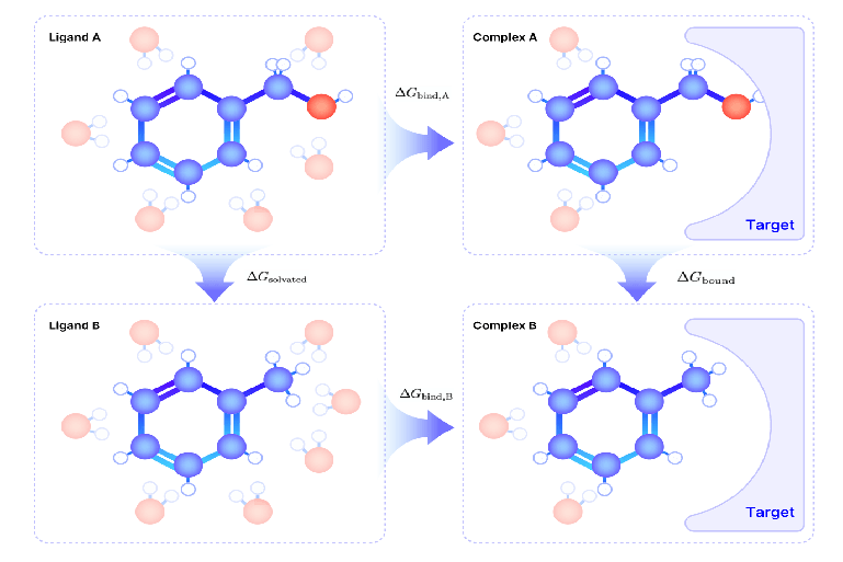
Fig.1 The Thermodynamic Cycle for Computing Relative Binding Free Energy Difference

In the solution environment, molecules A and B interact with solvent molecules, and their solvation free energy ($\Delta G_{solvation}$) can be calculated separately. In the binding environment, molecules A and B interact with the target protein, and their binding free energy ($\Delta G_{binding}$) are also calculated separately. However, directly calculating the absolute binding free energies of molecules A and B ($\Delta G_{binding A}$ and $\Delta G_{binding B}$) is extremely challenging since many factors, such as solvation effects and intermolecular interactions, need to be taken into consideration, which can lead to the accumulation of errors.

The thermodynamic cycle provides a solution to this problem. By calculating the relative free energy difference (ΔΔG)—the difference in free energy between molecules A and B in their solution and binding states—we can bypass the need to compute absolute free energies while achieving more stable and reliable results. According to the principles of the thermodynamic cycle, the total free energy change along two paths (solution and binding environments) is always equal:

$\Delta\Delta G = (\Delta G_{bind,B}-\Delta G_{bind,A})-(\Delta G_{solvated,B}-\Delta G_{solvated,A})$

To compute the free energy differences in the thermodynamic cycle described above, the FEP method was developed. The fundamental concept of FEP involves using Molecular Dynamics (MD) simulations to create a virtual "transformation pathway" between the molecule A and the molecule B. This pathway incrementally modifies the shape, properties, or chemical characteristics of molecule A into those of molecule B. Throughout this process, the free energy changes at each step are recorded, and these changes are then integrated using statistical mechanics formulas to compute the relative free energy difference between the molecule A and the molecule B. By following these steps, the FEP method enables efficient and reliable calculations of relative free energy in complex systems.

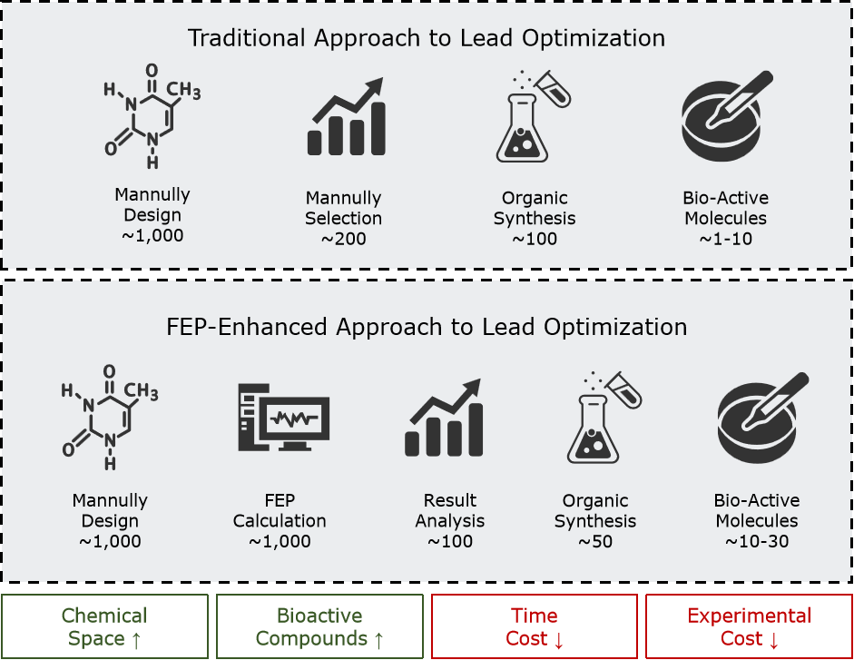
Fig.2 Improvements to the Lead Optimization Process Induced by FEP

Reflection: Why is FEP a Powerful Tool for Lead Compound Optimization? FEP calculations, with their near-chemical accuracy (typically achieving errors of less than 1 kcal/mol), have become a core tool in lead compound optimization. Compared to traditional methods that rely on chemical synthesis and experimental screening, FEP operates in a virtual environment, enabling the rapid evaluation of a large number of candidate molecules. This approach significantly expands the chemical space explored while reducing the time cost of the optimization process. By replacing experimental validation with computational screening, researchers can minimize the need for synthesizing and testing numerous compounds, allowing resources to be focused on the most promising molecules. This substantially enhances the chances of identifying more active compounds.

1.2 What Types of Projects are Suitable for FEP?

The core advantage of FEP lies in its ability to predict the relative binding free energy differences (ΔΔG) between similar molecules with near-chemical accuracy through MD simulations. A key step of FEP involves constructing a virtual "transformation pathway" between two molecules and simulating their relative transitions in both binding and solution states. The effectiveness of this approach depends on several factors, including the clarity of the binding mode in the target system, the extent of chemical differences between molecules, and the quality of experimental data supporting the computational model. Therefore, before applying FEP, the following conditions should be verified:

1. High-Quality Protein-Ligand Co-crystal Structure of the Target System

a. Resolution Better than 2.2 Å: The position of every amino acid residue and the ligand molecule in the system should be well-defined, with a structurally complete and detailed binding site.

b. Clear Ligand Binding Mode: The ligand molecule must form reasonable interactions with the protein (e.g., hydrogen bonds, hydrophobic interactions) and conform to the known binding mechanism. Additionally, the side chains of key amino acid residues in the binding site should not be missing and must have clearly defined positions.

Reflection: How to Address the Lack of High-Quality Co-Crystal Structures? When a system lacks high-resolution co-crystal structures, various modeling techniques can be combined to generate useful structural models. These techniques may include using AlphaFold to predict the protein structure, optimizing the binding conformation through molecular dynamic simulations, or employing molecular docking and induced fit docking methods to generate the initial binding conformation. However, all generated structures must undergo rigorous validation, particularly with regard to the ligand's binding mode in the binding site. It is essential to ensure that the binding interactions align with known mechanisms. If certain regions of the co-crystal structure are unresolved and distant from the binding site, computational tools can be used to complete those regions. For additional structural areas that are unrelated to ligand binding, simplification may be appropriate. In cases involving complex modeling requirements, it is advisable to consult a specialized computational biology team to ensure the reliability of the initial model and the accuracy of subsequent calculations.

2. Structural Similarity Among Ligands to Be Evaluated

a. Limited Range of Chemical Differences Between Ligands: All ligands in the set should form a continuous chemical space in terms of structure, with each molecule showing significant similarity to others in the set. Allowed chemical modifications include changes to substitution groups, scaffold hopping, adjustments to ring size or ring opening/closing withou significant changes to the overall shape.

b. Consistent Binding Mode Between Ligands and the Target Protein: All ligands in the set should form a consistent network of key interactions at the binding site (e.g., shared hydrogen bonds or π-π stacking). Shared key substructures should remain aligned in the binding conformation.

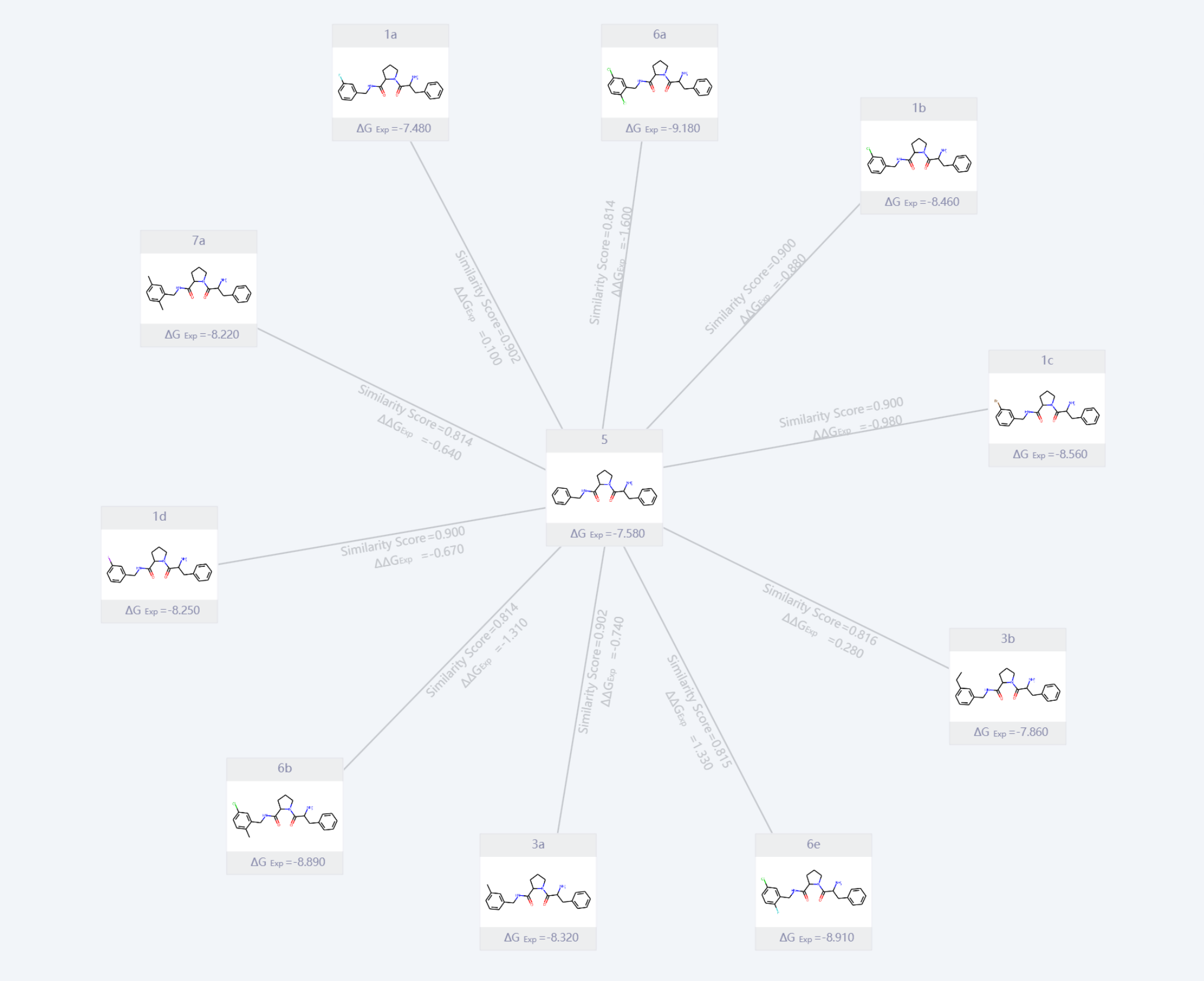
Fig.3 A set of Ligand Molecules with Similar Structure and Continuous Chemical Space

3. Some Ligands Have Reliable Experimental Data

a. Unified Source of Experimental Data: Experimental data must be obtained under consistent experimental conditions and batches, including the same experimental methods (e.g., SPR or ITC), protein sources, and buffer systems.

b. Wide Range of Binding Affinities in Experimental Data: Experimental data should cover a broad range of binding affinities, from weak to strong binding, for instance, IC50 values spanning from millimolar to nanomolar ranges.

Reflection: Why is it Necessary for Some Ligands to Have Reliable Experimental Data? Experimental binding affinity data play a dual role in FEP calculations: validation and calibration. Just as experiments require standard controls, computational methods must first be validated by experimental data to ensure their applicability to the target system before they are used for actual predictions. By performing calculations and comparisons on a set of molecules with known binding affinities, the prediction accuracy of FEP can be verified, and parameters can be adjusted to ensure the results align with experimental data. Only after confirming that the computational method can accurately capture the binding characteristics of the system can FEP be used for screening and optimizing new compounds. This process ensures the reliability of the calculations while enhancing the ability to predict the behavior of untested molecules.

Overall, FEP is a powerful computational tool, but its successful application depends on whether the system meets key conditions. If the system has high-quality structural data, the chemical properties of the ligand set are reasonable, and experimental data are sufficiently supportive, FEP can efficiently provide reliable predictive capabilities for lead compound optimization and molecular design.

In practical projects, if you are unsure whether the system meets the conditions for FEP applicability, you can use the guidelines in this article to evaluate each factor individually and consult with experts in your team or refer to existing literature models. If the conditions are preliminarily met, it is advisable to start with small-scale test systems, verifying prediction accuracy through benchmark tests, and then gradually expand the application scope. This approach ensures effective use of resources while minimizing risks in the model-building process.

Reflection: What Types of Projects Are Not Suitable for FEP? 1. Uncertain Protein-Ligand Binding Modes 2. Excessive Chemical Differences Among the set of Ligands 3. The Target Protein has Highly Complex Dynamic Characteristics

1.3 General Steps for Applying FEP to a Project

When applying the FEP method to a drug design project, it is typically divided into two phases: the validation phase and the production phase. This phased approach is designed to ensure the reliability of the model while optimizing resource utilization. In the validation phase, the focus is on testing the prediction accuracy of known ligands, confirming whether the FEP method is suitable for the target system, and constructing a usable FEP computational model. In the production phase, the validated model is used to predict the binding affinities of unknown molecules, supporting molecular screening and optimization efforts.

	Validation Phase	Production Phase
Input	A set of ligands with experimentally determined binding activity	A set of candidate ligands designed by medicinal chemists, for which activity has not yet been determined
Task	Validate the accuracy of the FEP computational model; Optimize the protein-ligand complex structure and simulation parameters	Use the validated FEP computational model to predict the binding free energy of the candidate molecules
Output	A validated FEP computational model	A list of top candidate molecules for experimental validation

Validation Phase: In the validation phase, researchers need to select a set of known ligands with experimental binding affinity data, ensuring that the data covers a range of binding affinities from weak to strong. The main objective of this phase is to assess the applicability of the FEP method to the target system, ensuring that the prediction results are sufficiently accurate and reliable. The model can be further optimized by adjusting parameters such as the force field, simulation conditions, and binding mode.

Specifically, the validation process begins by performing FEP simulations to calculate the relative binding free energy differences (ΔΔG) for the known ligands. These results are compared with experimental data, and statistical methods (such as RMSE and correlation coefficient R²) are used to evaluate the accuracy of the model.

As shown in the figure below, the x-axis represents the experimentally determined binding free energy ($ΔG_{exp}$), while the y-axis represents the FEP-calculated binding free energy ($ΔG_{FEP}$ ). The regression line in the plot indicates the linear fit between the calculated and the experimental values, while the error bars on the data points reflect the computational uncertainty for each molecule. The dark blue region represents a high-confidence interval (±1 kcal/mol), indicating a range where the computational results align closely with experimental data. The light blue region encompasses a broader uncertainty range (±2 kcal/mol). In general, if more data points fall within the dark blue region, it suggests lower prediction errors and higher overall accuracy of the model. If most data points deviate from the dark blue region, it may indicate model errors or parameter issues, requiring further optimization.

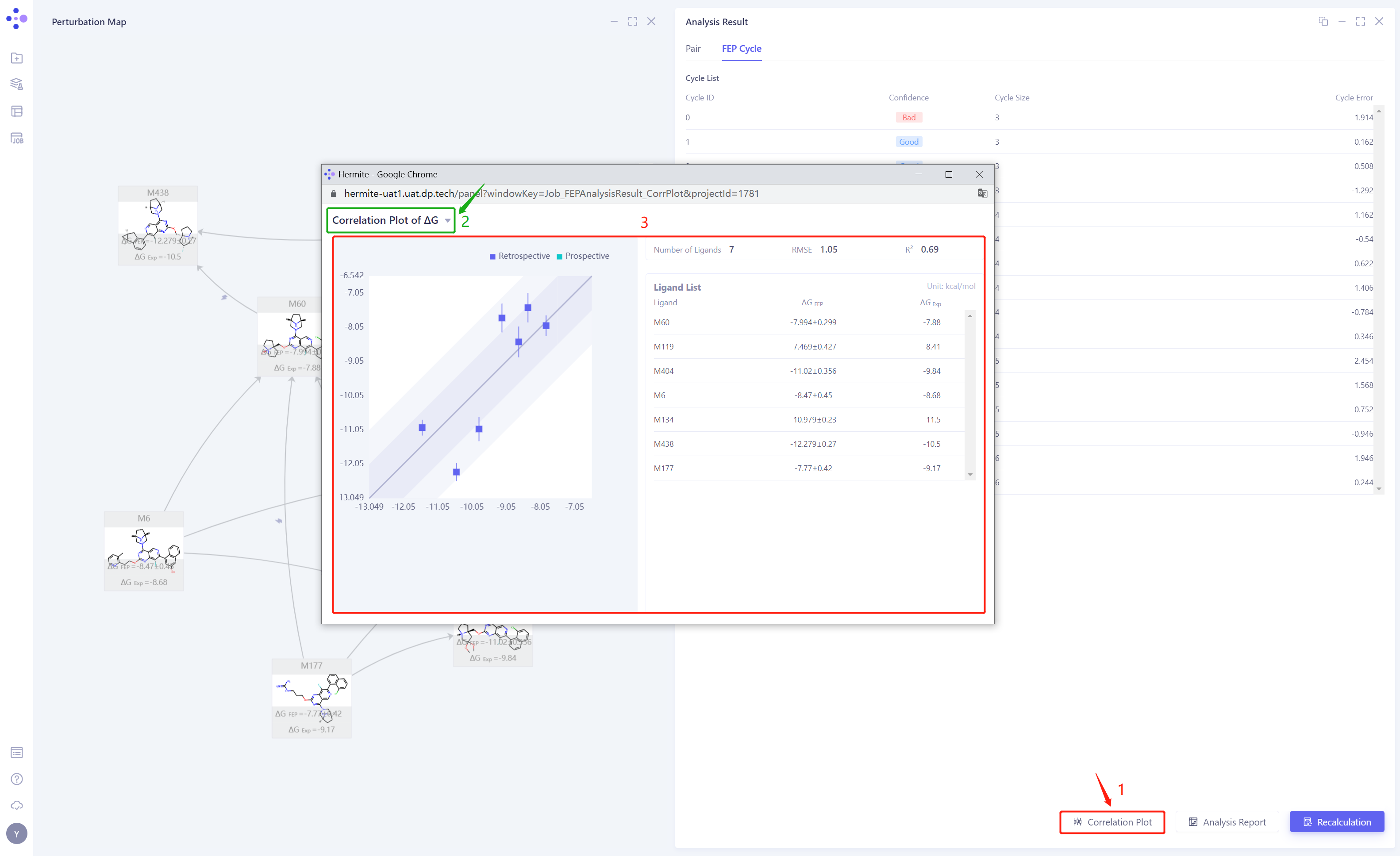
Fig.4 Correlation Plot Between FEP-Computed ΔG Values and Experimentally Measured Affinity Values

By iteratively optimizing the force field parameters, binding modes, and simulation conditions, the computational results are aligned with experimental data. Once the validation is completed, the constructed FEP computational model can be applied in the production phase, supporting subsequent molecular screening and design efforts.

Reflection: What is an FEP Computational Model? An FEP computational model refers to the complete system used for FEP calculations, including the essential components needed to construct the FEP method. Specifically, it includes the following parts: 1. Protein-Ligand Complex Structure: Pre-processed target protein structure and the ligand molecule’s binding conformation. It provides an accurate initial state for subsequent FEP calculations. 2. Simulation Parameters: Protein / Ligand molecular mechanics force fields and simulation conditions (such as temperature, solvent model, and path construction method) which are used to describe the target system.

Production Phase：With the validated FEP computational model, large-scale molecular screening or optimization efforts can be carried out. The input ligand set in this phase typically consists of a series of structural derivatives designed by medicinal chemists, starting from lead compounds. Through FEP calculations, the relative binding free energies (ΔΔG) of the candidate molecules are calculated individually, allowing for the selection of molecules with lower binding free energies and higher potential activity. These top candidates will undergo further experimental validation, while the computational results provide feedback for iterative molecular design.

The production phase leverages the highly accurate computational model from the validation phase to achieve efficient and reliable molecular screening, significantly narrowing the scope of experimental screening and improving the efficiency of drug development.

1.4 About Hermite® Uni-FEP

Hermite® is a next-generation drug design platform developed by DP Technology, powered by AI for Science, providing a comprehensive computational solution for preclinical drug development. It includes industry-leading tools including the free energy perturbation calculation tool Uni-FEP and ultra-high throughput virtual screening tool Uni-VSW, empowering various preclinical discovery stages such as protein structure prediction, target validation, lead compound discovery, and lead optimization.

Hermite® offers a web-based interactive molecular display experience, allowing fine-grained management of projects, team members, and data. The platform is equipped with complete certification and multi-layered security protection, supporting both online usage and private deployment. Hermite® is widely trusted by our customers, with over 60% of leading pharma companies in China choosing the platform and applied in more than 50 drug pipeline projects.

Tips: Hardware and Software Recommendations for Using the Hermite® Drug Design Platform Hardware: It is recommended to use a display monitor of 23.5 inches or larger for clearer visualization of protein-ligand complex structures, binding modes, ligand superimposition, perturbation diagrams, atomic mapping, and other related information. This will enhance modeling efficiency and analytical accuracy. A computer configuration with at least 8GB of RAM is recommended to ensure smooth software operation without lag. Software: The latest version of Google Chrome browser is recommended to ensure that all display components of the platform load correctly and run smoothly.

Uni-FEP is a computational drug design tool developed by DP Technology, based on the Free Energy Perturbation (FEP) theory, designed to accurately assess the binding affinity between proteins and ligands. Combining molecular dynamics, enhanced sampling algorithms, and AI-optimized molecular force fields, Uni-FEP has been validated on over 50 protein systems, achieving industry-leading performance. With high-performance computing optimization, a single FEP calculation under recommended parameters can be completed in approximately 4 hours. Leveraging massive cloud computing power, Uni-FEP can perform parallel calculations of thousands of FEP tasks simultaneously.

Additionally, Uni-FEP offers a browser-based intuitive visualization interface that allows users to inspect and adjust molecular structures, protein-ligand complex binding modes, freely build and edit perturbation graphs and atomic maps, and analyze FEP results from multiple dimensions, providing an industry-leading interactive experience. Clients have completed over 200,000 Uni-FEP calculation tasks on the Hermite® platform.

Tips: Case Studies on Computational Accuracy Verification of the Hermite® Uni-FEP Module Chapter 6 provides detailed case studies demonstrating the accuracy of binding free energy calculations with the Hermite® Uni-FEP module. Interested readers can refer to Chapter 6 for more details. In the verification system [1] (a total of 8 protein-ligand sets and 199 ligand molecules), Uni-FEP achieved a correlation coefficient (R²) of 0.56 and a root mean square error (RMSE) of 0.89 kcal/mol after 5ns of simulation. In verification system [2] (a total of 8 protein-ligand sets and 264 ligand molecules), Uni-FEP achieved an R² of 0.41 and an RMSE of 1.23 kcal/mol after 5ns of simulation. These tests demonstrate the industry-leading computational accuracy of Uni-FEP. [1] Wang, Lingle, et al. "Accurate and reliable prediction of relative ligand binding potency in prospective drug discovery by way of a modern free-energy calculation protocol and force field." Journal of the American Chemical Society 137.7 (2015): 2695-2703. [2] Schindler, Christina EM, et al. "Large-scale assessment of binding free energy calculations in active drug discovery projects." Journal of Chemical Information and Modeling 60.11 (2020): 5457-5474.

The Hermite® Uni-FEP module is a drug design tool specifically designed for free energy perturbation calculations. It consists of three main pages: FEP task submission, FEP task management, and FEP result analysis. Uni-FEP provides interactive features such as a 3D structure panel for complexes, a plane panel for perturbation graphs, atomic mapping for 2D validation and 3D modification, among others. It supports a one-stop solution for system preparation, perturbation graph construction, atomic mapping verification, simulation parameter setting, task management, result visualization, and binding free energy statistical analysis, covering all aspects to perform FEP calculation tasks.

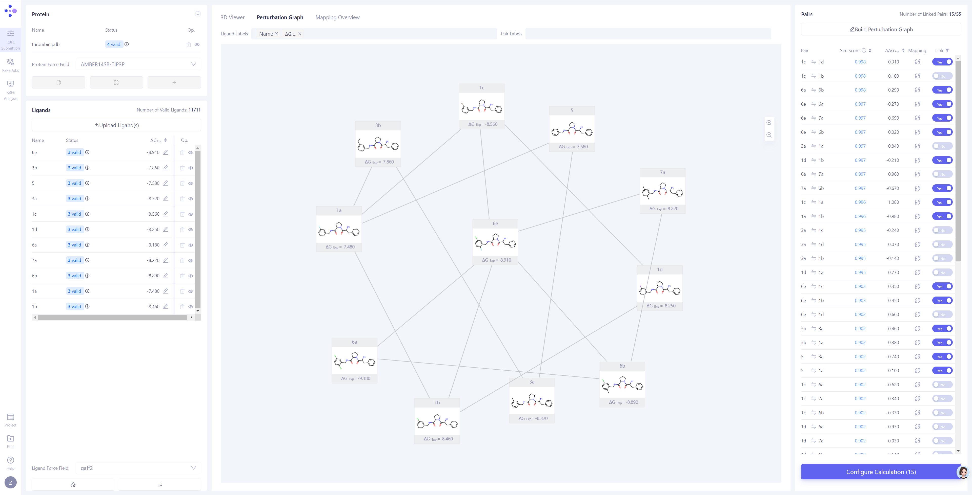
Fig.5 Hermite®️ Uni-FEP Task Submission Interface

2. Using Uni-FEP for Relative Free Energy Calculations – Step-by-Step Guide

Tips: For Readers Unfamiliar with FEP Calculations, Please Skip This Chapter This chapter is designed to provide a clear and concise guide for users already familiar with FEP calculations, ensuring that each important step is properly followed. If you're new to FEP calculations, we recommend starting with Chapter 3. This chapter includes case studies and visual interface screenshots that will help you understand how to complete a full calculation and analysis using the Hermite Uni-FEP platform. Afterward, you can use the content of this chapter as a step-by-step guide for practical application.

2.1 FEP Data Collection and Basic Checks

1. Collect and Inspect Protein Structures

• Select high-quality co-crystal complex structures as the starting protein model, ensuring that the amino acid residues near the binding pocket are clearly resolved and that no protein chains are broken.

• Verify that the reference ligand forms reasonable interactions with the binding pocket.

2. Collect and Inspect Molecular Structures and Properties

• Ensure that ligands in the molecule set share structural similarities with the reference ligand, and that the binding mode in the binding pocket is consistent with that of the reference ligand.

• Confirm that some molecules in the set have reliable experimental data, with consistent data sources covering a broad range of binding affinities.

2.2 FEP System Preparation and Task Submission

1. Upload the Protein and Perform Protein Preparation

• Upload the protein file and perform basic protein preparation and automatic checks. If any issues are detected, correct the structure based on feedback.

• For residues in the binding pocket with protonatable side chains, adjust the protonation state based on predicted pKa values and their interactions with the ligand and water molecules.

• If the binding mode is influenced by cofactors, upload the cofactor structure or the pre-constructed force field file.

• If the target protein is a membrane protein, select appropriate parameters to build the membrane structure.

2. Upload Ligand Molecules and Perform Ligand Alignment

• Upload the ligand molecules and perform automatic ligand checks. If issues arise, modify the ligand structure based on feedback.

• For ligands that do not align with the reference molecule, set a common scaffold with the reference molecule to perform ligand alignment. If ligand the alignment is poor or the aligned conformation clashes with the protein structure, modify the scaffold or choose another reference molecule until all ligands form a consistent and reasonable binding mode.

• If the ligand molecules have experimentally determined binding affinity data, import that data.

• In most cases, it is recommended to enable the automatic optimization of the small molecule force field parameters. After optimization, inspect the results and decide whether to use the optimized force field.

3. Build the Perturbation Graph and Check Atom Mapping for the Molecules to Be Computed

• Based on the ligand molecule information, update the perturbation molecule pair list.

• Automatically generate the perturbation graph, or manually construct it based on molecular similarity, ensuring that each ligand molecule is connected to at least one structurally similar molecule.

• Carefully check the atom mapping for each molecule pair to ensure a one-to-one correspondence of atoms in the shared structure.

4. Set Computational Parameters and Submit the Task

• Enter the confirmation page before submission and verify that the selected protein and the molecule pairs to be computed match expectations.

• Review and confirm the FEP simulation parameters to ensure correct simulation settings.

• Ensure the available FEP pairs are sufficient to complete the computation by checking the account balance.

• Click Submit, and the FEP computation task will be automatically assigned to the computing cluster.

2.3 FEP Task Monitoring and Result Analysis

1. Monitor Task Progress and Status

• In the FEP task interface, track the progress and status of each molecular pair simulation.

• If a simulation for a particular molecular pair fails, review and adjust its atom mapping or simulation parameters, considering resubmission.

2. Analyze Individual Molecular Pair Calculation Results

• After the simulation task completes, expand the specific results to check if the simulation has converged.

• If the simulation has not converged, consider resubmitting or extending the simulation time.

• If multiple simulation records exist for a molecular pair, choose the optimal result based on convergence for further analysis.

3. Summarize All Molecular Pair Calculation Results

• Navigate to the FEP analysis interface to assess which molecular pairs should be retained for final analysis, based on the quality of the thermodynamic cycle.

• Use correlation plots to evaluate the relationship between FEP-calculated binding free energy and experimental data, assessing the credibility of the FEP computational model.

• Based on the FEP results, gain rational insights into molecules with undetermined activity.

2.4 Using Uni-FEP for Relative Free Energy Calculation - Example of the Thrombin System

Thrombin is an enzyme that plays a key role in blood coagulation. In the blooding cotting process, it converts fibrinogen into fibrin, forming a blood clot. Inhibiting or regulating the activity of thrombin can directly affect the blood clotting process. Therefore, developing small-molecule inhibitors for thrombin is crucial for the treatment of thrombotic diseases and anticoagulants.
In this section, we will demonstrate how to use Uni-FEP for free energy perturbation calculations, including system construction and validation, using thrombin as the target based on a reported drug development project. This case is derived from the study by Bernhard Baum et al. published in the Journal of Molecular Biology on 2009[1], which explores the binding mechanism of drug molecules in the thrombin S1 specificity pocket. Using X-ray crystallography and other experimental techniques, the study revealed the critical contribution of interactions formed by key residues such as Asp189 and Tyr228 to the binding free energy.

[1] Baum B, Mohamed M, Zayed M, Gerlach C, Heine A, Hangauer D, Klebe G. More than a simple lipophilic contact: a detailed thermodynamic analysis of nonbasic residues in the S1 pocket of thrombin. Journal of molecular biology. 2009 Jul 3;390(1):56-69.

2.5 FEP Data Collection and Basic Checks

The example data used in this tutorial can be downloaded via the link: https://bohrium-api.dp.tech/ds-dl/uni-fep-tutorial-j234-v1.zip.

2.5.1 Collect and Check the Protein Structure

We selected the 2ZFF crystal structure as the reference model. This structure resolves the complex of Thrombin protein with the unsubsituted phenyl inhibitor 5, with a resolution of 1.47 Å. It provides a clear and high-quality conformation of the binding pocket, especially the spatial positioning of key residues in the S1 specificity pocket, such as Asp189 and Tyr228. This provides a reliable starting protein structure for FEP calculations and ensures that the interaction patterns within the binding pocket are highly credible.

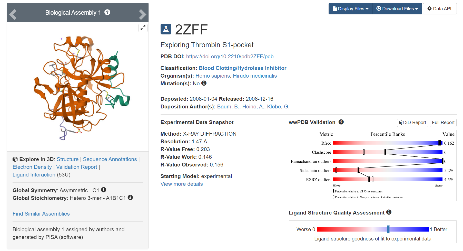
Fig.6 The Co-crystal Structure of the Thrombin Protein and its Inhibitors (PDB ID: 2ZFF)

2.5.2 Collect and Check the Molecular Structures and Properties

We selected a series of inhibitors with similar structures but different substitutions, including 1a, 1b, 1c, 1d, 3a, 3b, 5, 6a, 6b, 6e, and 7a in the below figure. These molecules retain a core scaffold that shares a highly consistent binding mode to the target protein, while the phenyl substitution in the S1 pocket exhibit systematic variations, such as chlorine, fluorine, bromine, and methyl groups, which reflect the contributions of hydrophobicity, volume, and specific interactions to the binding affinity. In addition, these molecules cover a broad range of experimentally determined binding free energy, providing comprehensive and consistent thermodynamic data to support the validation of the FEP model.

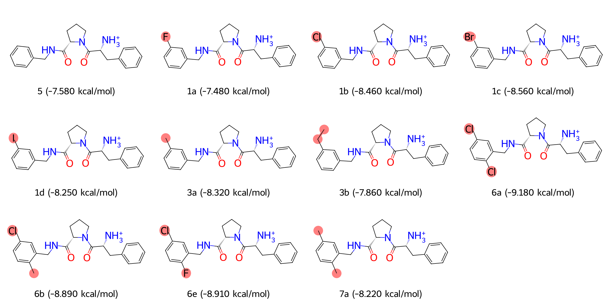
Fig.7 Structures and Binding Free Energy Values of Thrombin Protein Inhibitors

2.6 FEP System Preparation and Task Submission

2.6.1 Create a FEP Project and Enter the Project Page

Operation Description	Interface Screenshot
On the Hermite project list page, click the + New button in the top-right corner, enter the project name (e.g., "Tutorial_Thrombin"), select "FEP" as the project type, and then click Apply to create a FEP project and enter the project page.

2.6.2 Uploda and Prepare the Protein and Perform Protein Check

Protein preparation is a crucial step in FEP calculations to ensure the validity, accuracy, and stability of the protein structure. This section will guide you through the steps of uploading the protein, performing structural checks, and making protonation adjustments.

Operation Description	Interface Screenshot
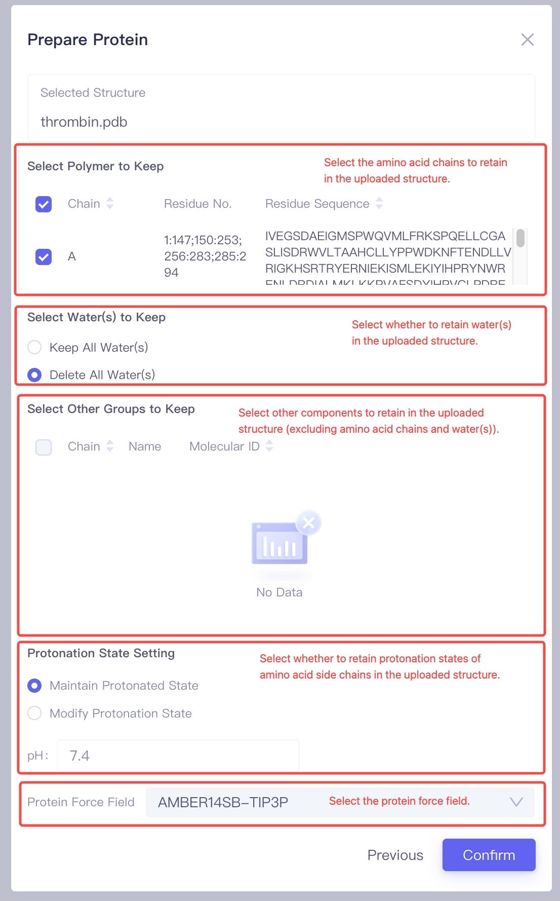
Upload the Protein Structure File and Perform Preparation: In the protein panel at the top left of the page, click the Upload a Protein button, select the protein structure file to upload (e.g., thrombin.pdb), and then click Next to proceed to the protein preparation interface. Select the Amino Acid Chains to Keep: In the "Select Polymer to Keep" option, choose the amino acid chains to Keep. Generally, the chains related to the ligand binding site should be kept to ensure the accuracy of subsequent calculations. Select the Water Molecules to Keep: In the "Select Water(s) to Keep" option, decide whether to keep the water molecules in the crystal structure. If the uploaded structure contains: (1) Water molecules buried inside the protein that are important for the overall structural stability; (2) Water molecules involved in protein-ligand interactions; It is recommended to select "Keep All Water(s)". Otherwise, choose "Delete All Water(s)" to remove water molecules and reduce computational burden. Select Other Molecules or Chemical Groups to Keep: In the "Select Other Groups to Keep" option, check if there are other molecules or chemical groups that need to be kept (e.g., cofactors, covalent modification groups, etc.). Adjust Protonation States of Amino Acid Side Chains: In the "Protonation State Setting" panel, choose the protonation state settings. If you have already confirmed the protonation states of each amino acid, use "Maintain Protonated State" to preserve the protonation states of the amino acid side chains from the crystal structure. Alternatively, you can select "Modify Protonation State" to let the program automatically adjust the protonation states based on the pH value you set. Select the Protein Force Field: In the "Protein Force Field" section, choose an appropriate force field (e.g., "AMBER14SB-TIP3P") to ensure accurate and reliable energy calculations for the protein during molecular dynamics simulations. Confirm Protein Structure Settings: After completing the above settings, click the Confirm button, and the system will begin preprocessing the protein structure and performing validity checks. This process typically takes about one minute.
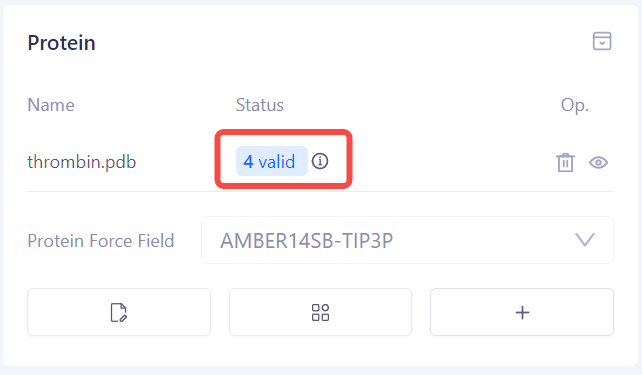
Check Protein Preparation Status: Once the protein preparation is completed, the system will display the status of the check, including "Valid", "Warning", or "Error". You can make corrections or perform further checks based on the provided prompts.
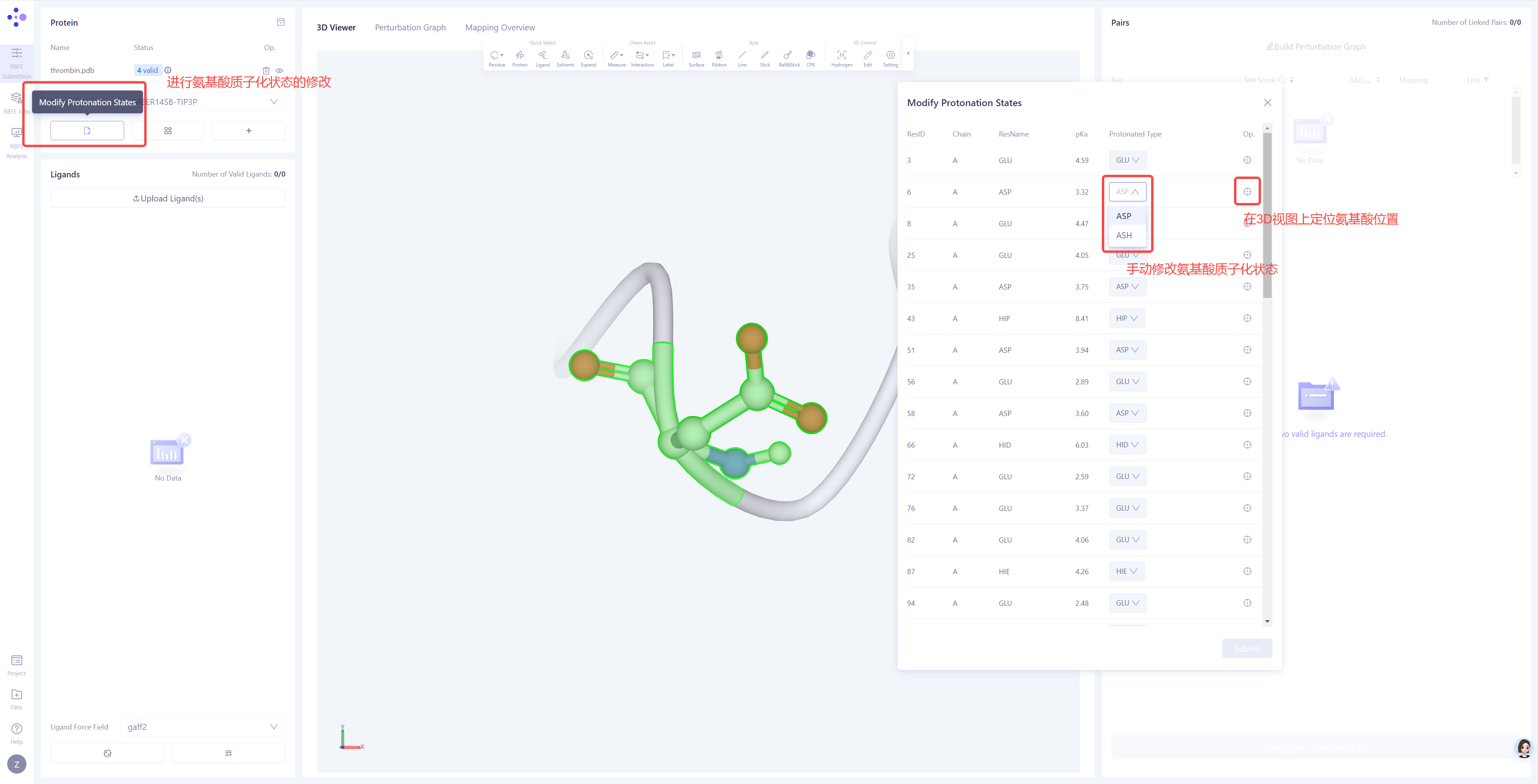
Manually Adjust Protonation States: If there are warnings regarding protonation states in the check results or if there are important protonatable amino acids near the protein-ligand binding site, you can click the Modify Protonation States option to manually inspect and adjust the protonation states.
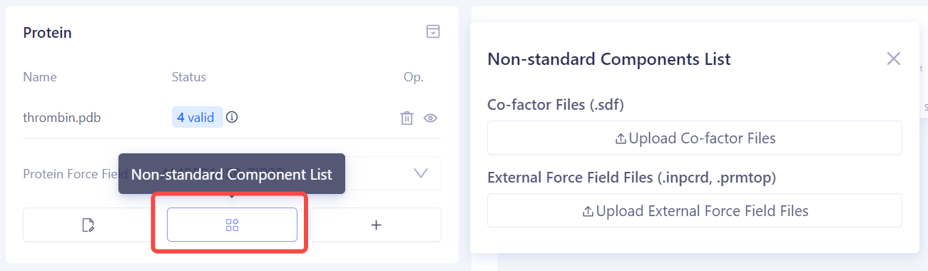
Add Non-standard Components: If there are non-standard components (such as co-factors or metal ions) near the protein binding site, upload the relevant ligand structures or pre-built force field parameter files in the Non-standard Components List to ensure the accuracy of the simulation.
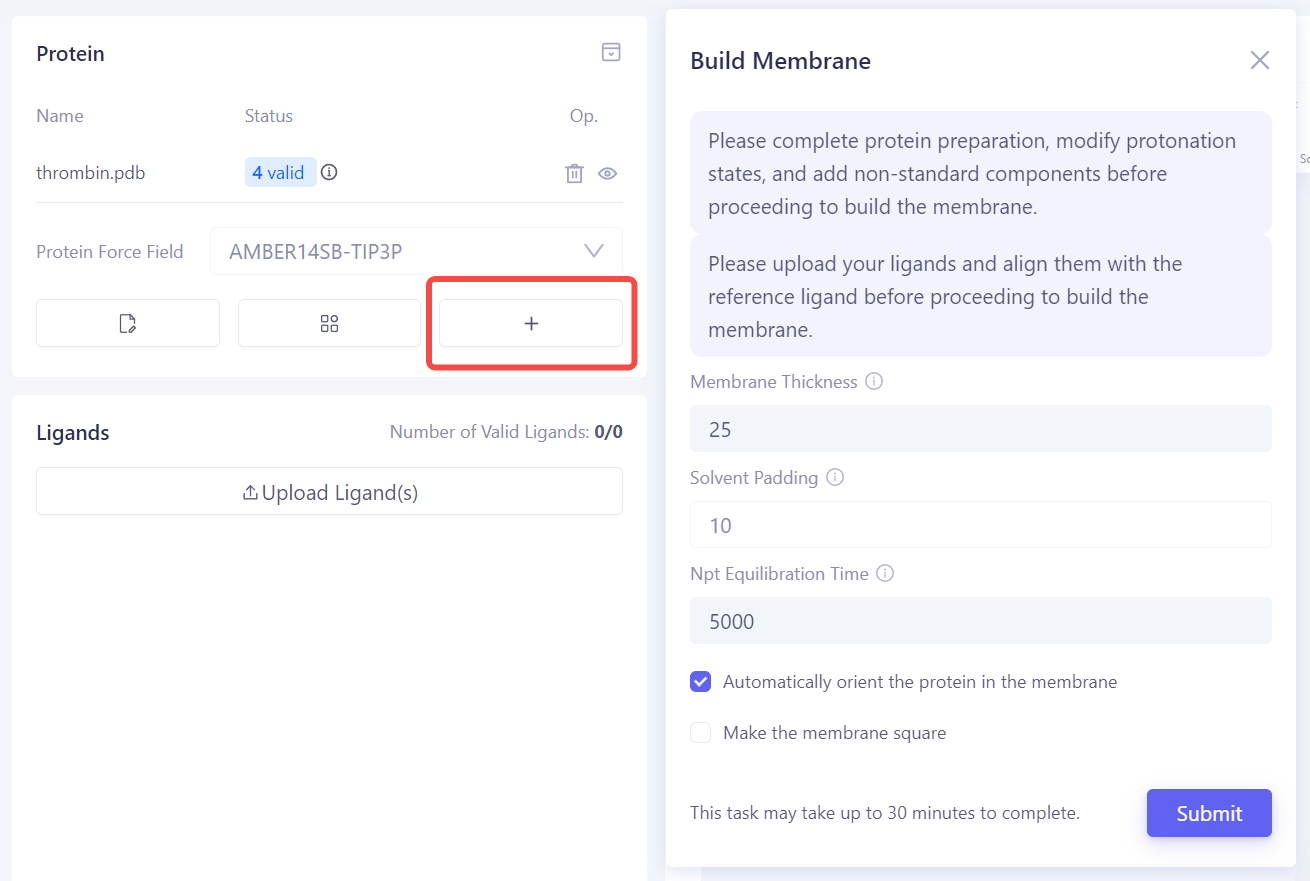
Build the Membrane Environment: If the target protein is a membrane protein, click Build Membrane to enter the membrane construction interface. In this interface, you can adjust parameters such as the thickness of the membrane, solvent filling layer, and equilibration time to ensure the protein is properly embedded in the membrane.
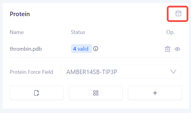
Fold the Protein Panel: After completing the above steps, you can click the Fold button to hide the protein setup components and save screen space.

Tip: Items for Protein Validity Check and Possible Statuses Collision Check (Valid/Error): Checks for unreasonable atomic collisions in the protein structure. Common issues include atomic overlaps, non-physical proximity, unusual replaceable residues, and metal ions that are not coordinated. These problems may lead to instability in simulations or failure in the energy minimization. Bond Length Check (Valid/Error): Verifies that all chemical bond lengths in the protein are within a reasonable range to avoid unnatural stretching or compression, ensuring stability in molecular dynamics simulations. Backbone Dihedral Angle Check (Valid/Warning): Examines whether the backbone dihedral angles of the protein lie within a reasonable conformational space (such as the allowed region in a Ramachandran plot) to avoid unnatural backbone conformations that may affect structural stability. Coplanarity Check (Valid/Warning): Validates whether specific atoms on a planar ring are free from unreasonable distortion or deviations from coplanarity, especially in aromatic rings, conjugated planes, or specific residues (e.g., proline). These abnormalities can affect the accuracy of energy calculations. Force Field Parameter Check (Valid/Error): Ensures that all components of the protein structure have complete and appropriate force field parameters for accurate interaction energy calculations in subsequent molecular dynamics simulations. Protonation State Check (Valid/Warning): Ensures that protonation states of amino acid residues and ligands in the protein are reasonable under the specified pH conditions, especially at the active site residues (e.g., histidine, glutamic acid, aspartic acid), to avoid invalid charge distribution that could impact binding free energy calculations.

2.6.3 Upload Ligand Molecules and Perform Ligand Alignment

Ligand preparation is a critical pre-step for performing FEP calculations, ensuring the validity, accuracy, and proper spatial alignment of the ligand molecules with the reference ligand. This section will guide you through the steps for uploading, checking, aligning ligands, and importing experimental data.

Operation Description	Interface Screenshot
Upload Ligand Structure File: In the Ligand Panel at the top left of the page, click the Upload Ligand(s) button, and select the ligand structure file to upload (e.g., 1a.sdf). The system will automatically perform a validity check on the ligand. If the uploaded .sdf file contains multiple ligands, the system will automatically split them into separate ligand entries.
Check Ligand Validity: After the ligand check is completed, the system will display the check results status, including "Valid", "Warning", or "Error". You can make corrections or further reviews based on the provided feedback.
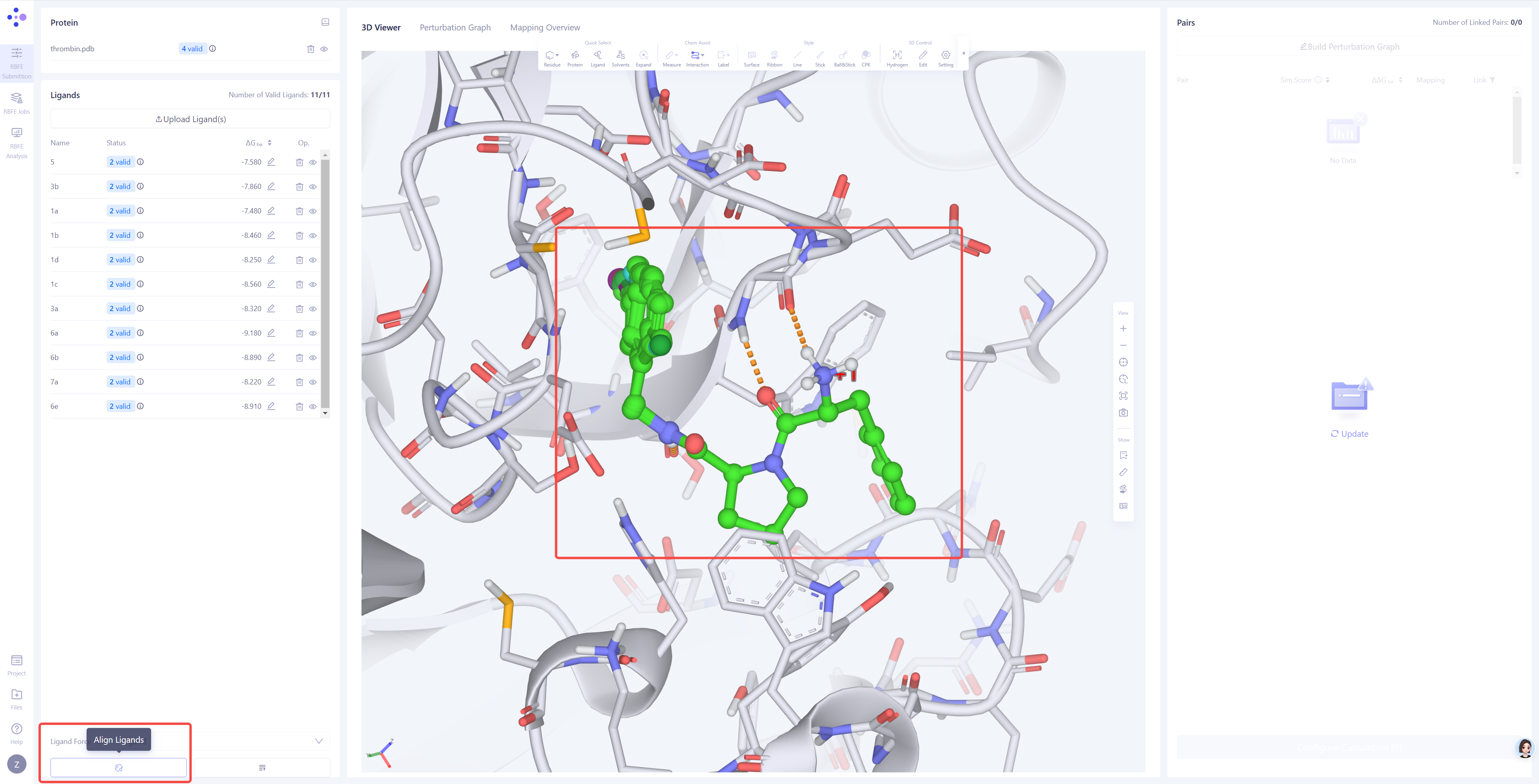
Ligand Alignment: In the 3D panel, check whether the uploaded ligands are properly aligned with the reference ligand. If ligands are not well-alignmed to the reference ligand , click the Align Ligands button in the bottom-right corner to perform the alignment. Select the Reference Ligand: Choose a reference ligand structure that has formed reliable interactions with the protein, ensuring it can serve as the basis for alignment. Then click Next. 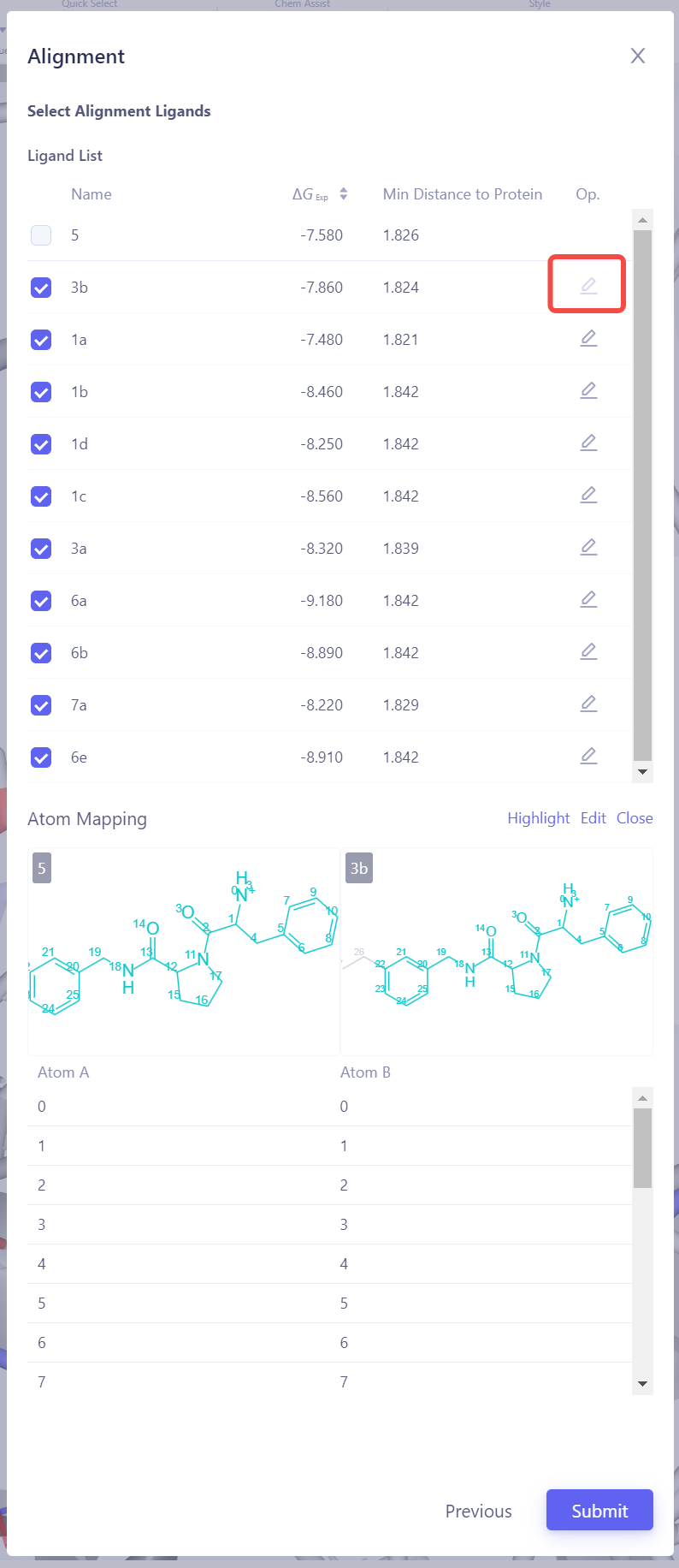Select Target Ligands: Select other ligands to be aligned with the reference ligand. Click "Atom Mapping" to check and confirm the atom mapping, and manually adjust it if necessary. Submit Alignment Task: After confirming all settings are correct, click Submit to start the ligand alignment task. Verify Alignment Results: After the alignment task is completed, check the alignment result of all ligands in the 3D panel. If the alignment is not ideal, try using a different reference ligand or adjust the atom mapping settings, then realign until all ligands achieve a good alignment.
Upload Experimental Binding Affinity Data: If the ligand molecules have experimentally determined activity data (such as IC₅₀ or Ki values), you can directly edit the corresponding experimental values for the respective molecules in the system, or click the Upload Affinity Data button in the bottom-right corner to batch upload experimental data using a template file, ensuring that the experimental values are correctly linked to the ligand molecules.

Tips: Ligand Molecule Validity Check Items and Possible Statuses Ligand-Protein Distance Check (Valid/Warning): This check evaluates the spatial distance between the ligand and the protein to ensure the ligand is in a reasonable binding site. It avoids non-physical proximity or excessive distance of the ligand to the bindning site, which could lead to deviations in binding free energy calculations.

2.6.4 Constructing the Perturbation Graph and Checking Atom Mapping for Molecule Pairs

Contructing the perturbation graph and checking the atom mappings are important steps before performing FEP calculations, ensuring that connections between molecule pairs are reasonable and the atom mappings are accurate. This section will guide you step by step on how to construct the perturbation graph and check the atom mappings.

Operation Description	Interface Screenshot
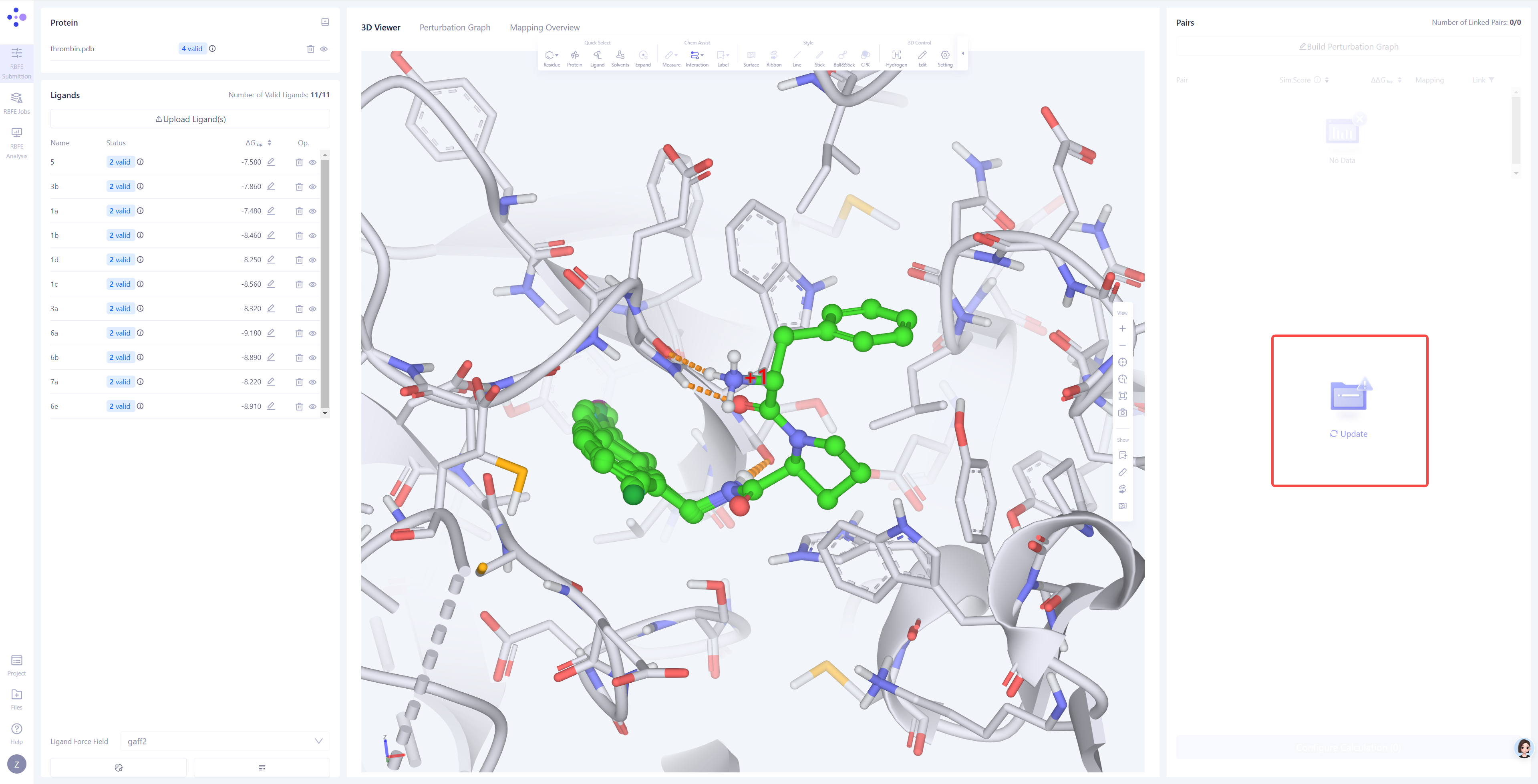
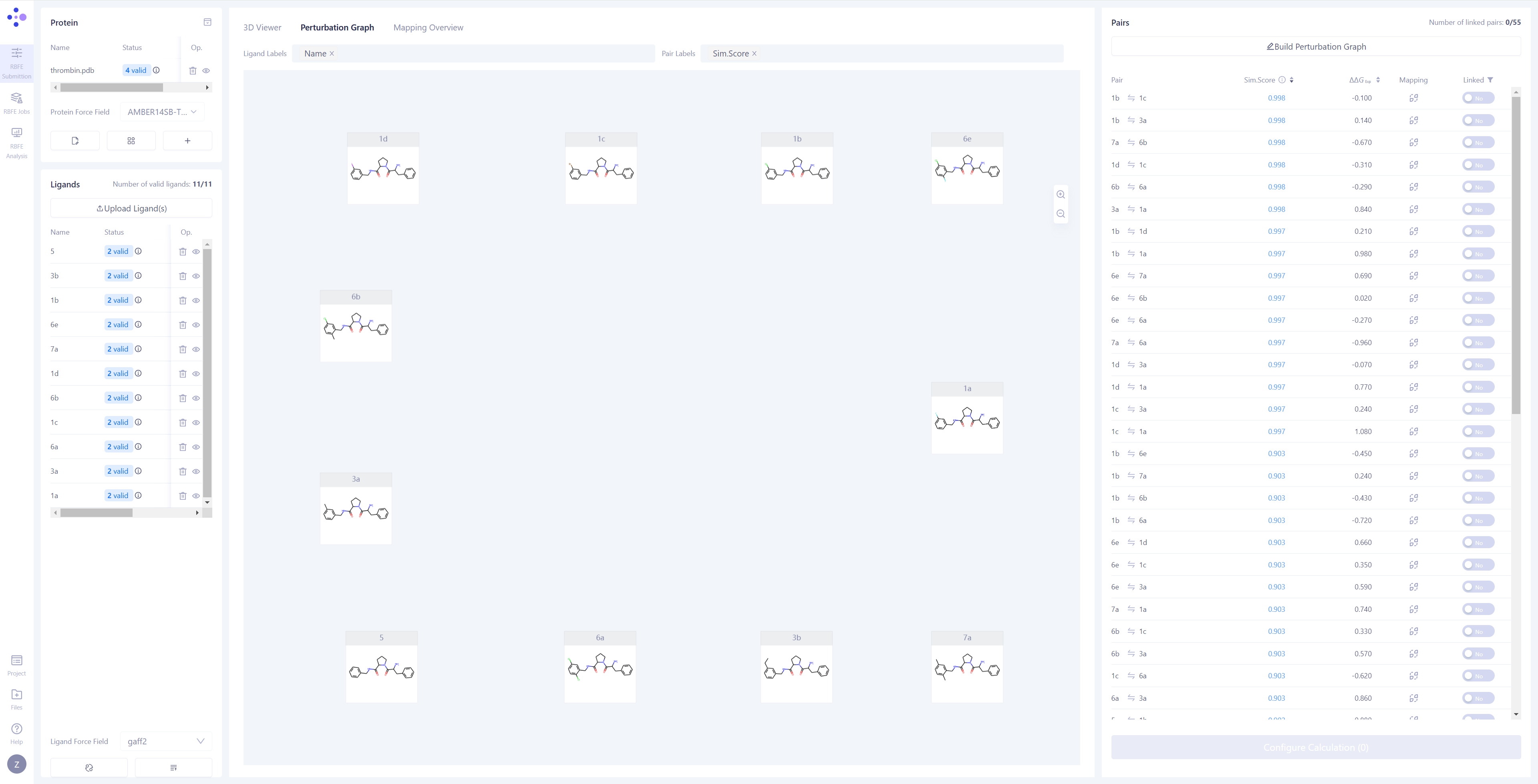
Updating Molecule Pair Information: In the "Molecule Pair" pane on the right, click the Update button. The system will automatically perform 3D atom mapping in pairs for all molecules detected as "Valid" and synchronize the result to the form. This process will take approximately 1 minute.
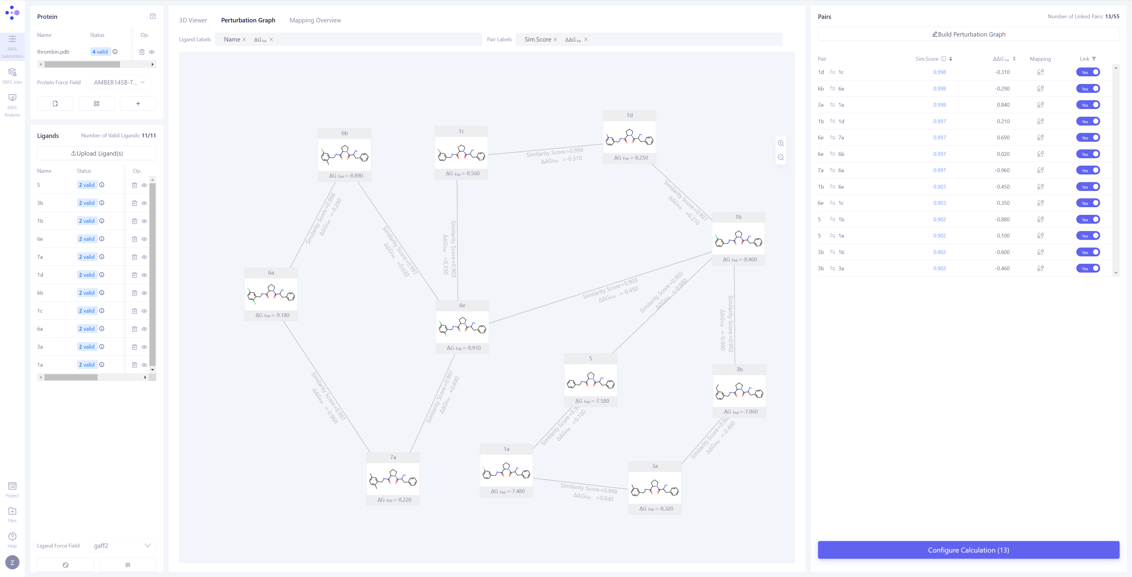
Constructing the Perturbation Graph: Once the synchronization is completed, the center view will automatically switch to the "Perturbation Graph" page. You can choose to manually connect the perturbation pairs you want to compute, or click Build Perturbation Graph to automatically construct the perturbation graph. Automatically Build the Perturbation Graph: Click the Build Perturbation Graph button to open the automatic construction settings window. Select all the molecules to be included in the calculation. If you wish to build a star-shaped perturbation graph (i.e., using one ligand molecule as the center, connecting it to all other molecules), enable the "Build star-shaped perturbation graph" option and select the central ligand. Click the Submit button, and the system will automatically generate the perturbation graph. Filter Linked Edges: In the "Linked" list in the upper right corner, select the "Yes" option to quickly filter and view all the connected edges and their related information.
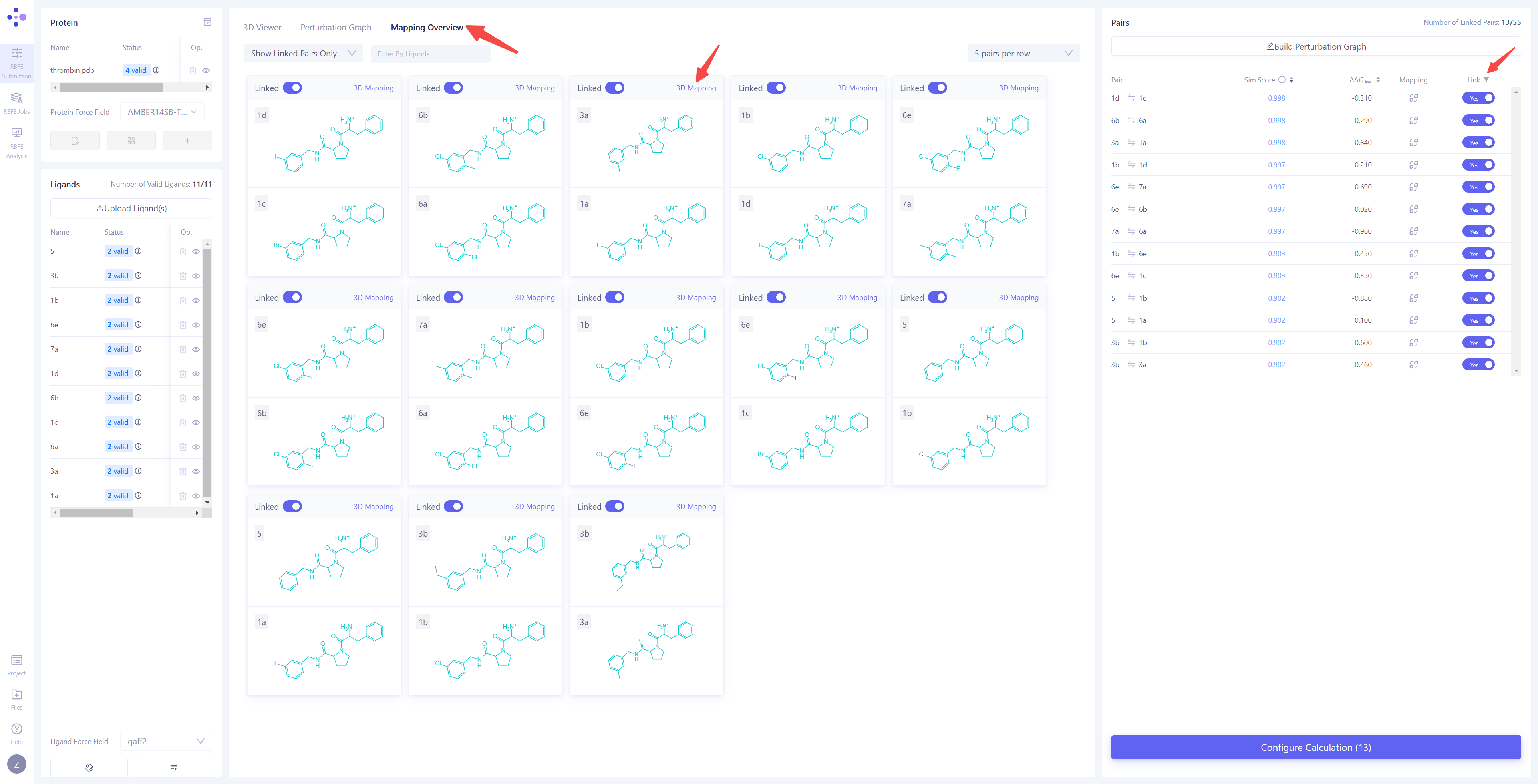
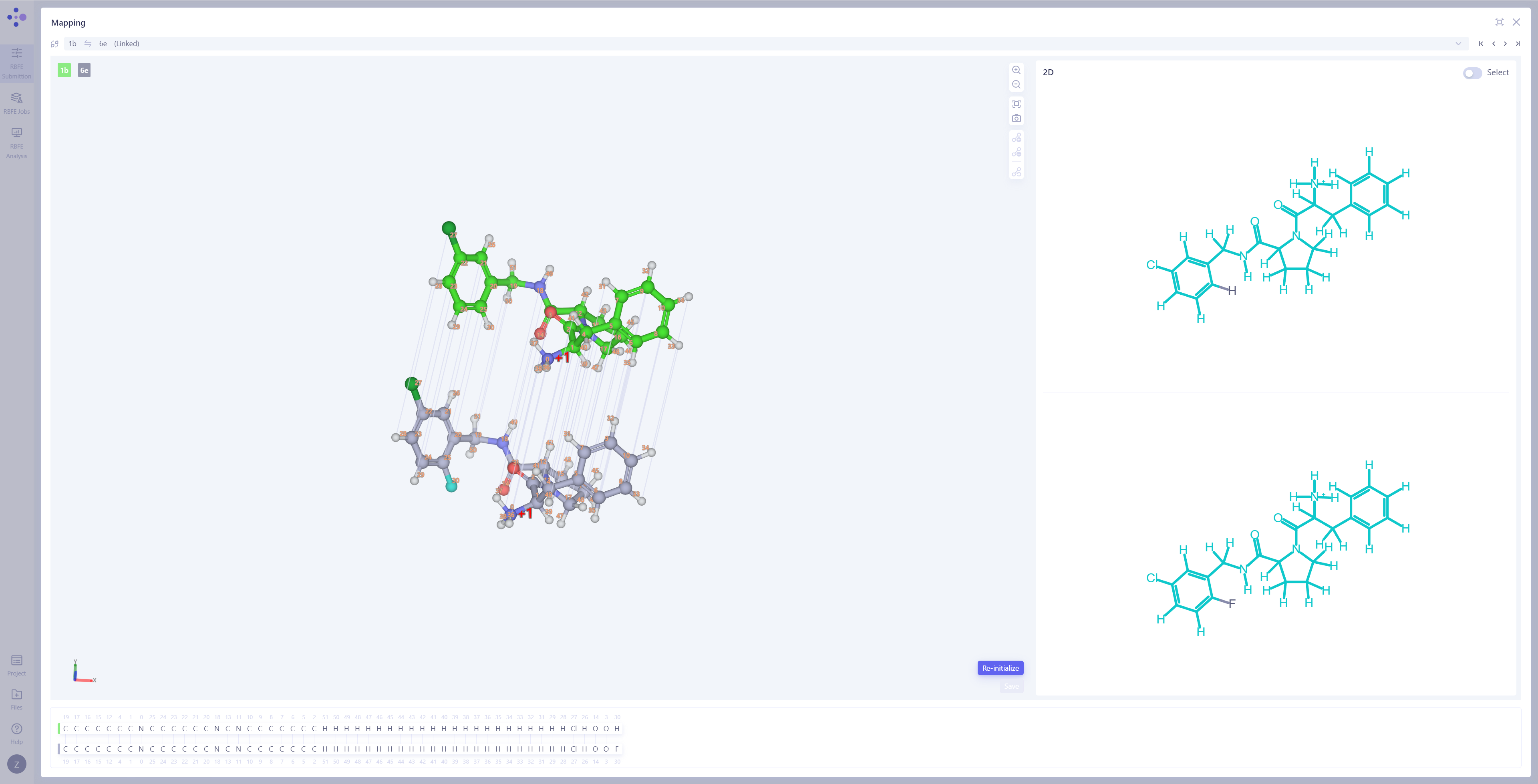
Check Atom Mapping: Switch the center view to the "Mapping Overview" mode to check the atom mapping of all connected edges, ensuring the accuracy and completeness of the mapping. Inspect Atom Mapping Details: If you find incorrect mappings or need to further examine specific atom pairs, click "3D Mapping" to open the atom mapping details interface. Modify Atom Mapping: In the 3D Mapping panel, you can perform the following actions: directly select atom pairs in the 3D view to add or remove atom mappings; in the 2D mapping view on the right, perform bulk mapping operations by selecting regions of the molecule; in the atom numbering mapping area at the bottom, make large-scale adjustments by selecting atom indexes. After completing all operations, click Save to save the modified atom mappings.

2.6.5 Set Calculation Parameters and Submit Calculation Tasks

Operation Description

Interface Screenshot

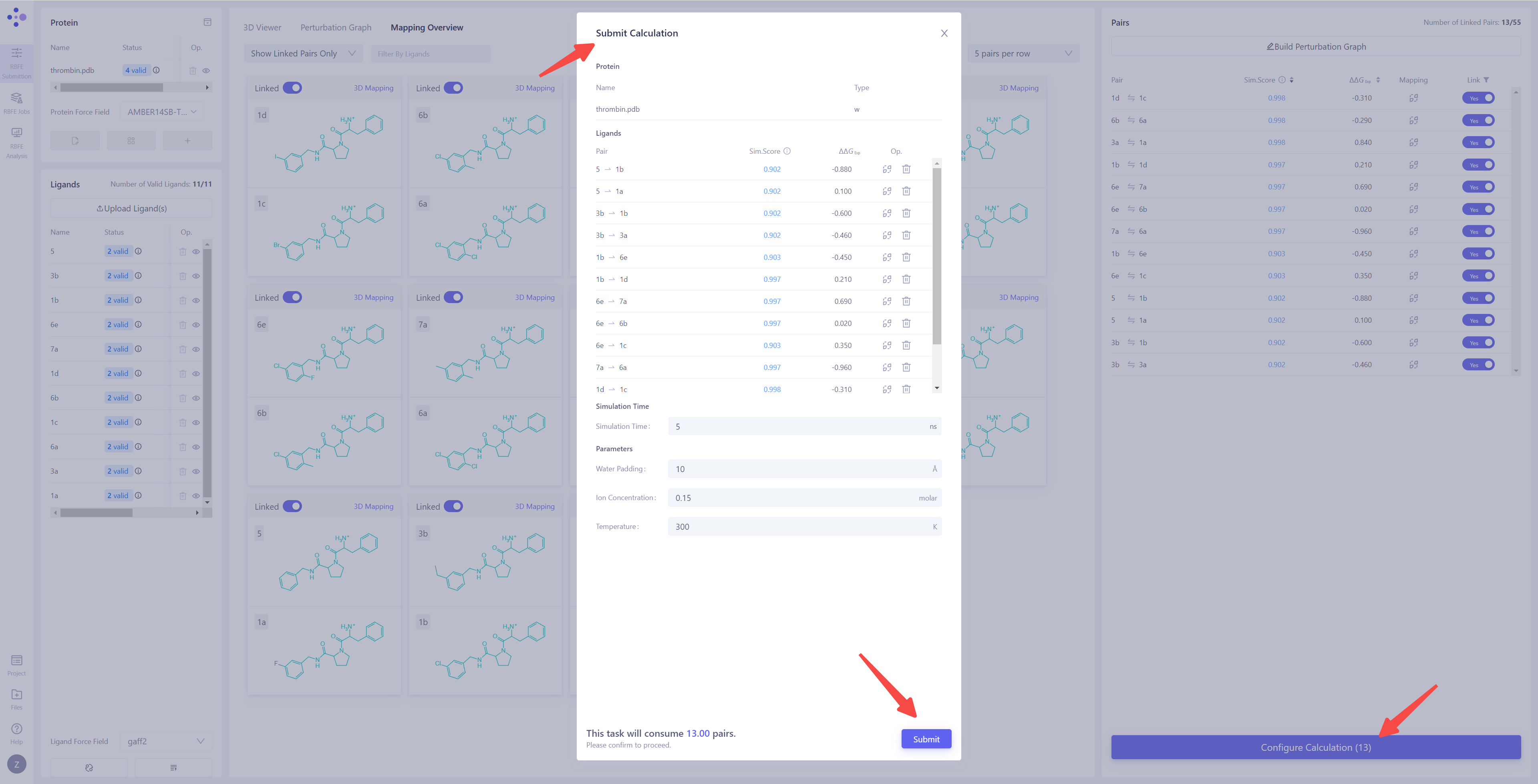
Enter the Calculation Parameters Configuration Interface: Once all prerequisite tasks are completed, the Configure Calculation button in the lower-right corner will become clickable. Click this button to enter the FEP calculation parameters configuration interface and begin the detailed task setup. Confirm the Membrane Protein System Identification: If the target system is a membrane protein, ensure that the "Type" column is marked as "with Membrane" to ensure that the simulation conditions correctly match the membrane environment. Check Perturbation Pairs: Ensure that all perturbation pairs are as expected. You can click "Mapping" to perform a secondary check of the atom mappings and verify their accuracy. If there are perturbation pairs that should not be included in the calculation, you can select the corresponding entries and click "Delete" to remove them. Set Simulation Time: For common systems, it is recommended to set the simulation time to 5 ns to ensure the stability and accuracy of the results. Configure Simulation Parameters: Set the water padding to ensure that the system boundary does not interfere with the simulation results. Set the ion concentration and set the ion type as Na⁺ and Cl⁻ ions to neutralize the system's charge and simulate physiological conditions. Set the simulation Temperature to 300 K, which is commonly used to match typical experimental conditions. Confirm Calculation Cost: After all parameters have been set, the system will automatically estimate the cost of the current batch of FEP calculations. Please carefully review all settings and calculation resource information to ensure there are no errors. Submit the Calculation Task: Click the Submit button to submit all FEP calculation tasks to the server and begin the official computation.

2.7 FEP Task Monitoring and Result Analysis

2.7.1 Monitoring Task Progress and Status

Operation Description	Interface Screenshot
Enter the FEP Task Management Interface: In the left sidebar, click "RBFE Jobs" to enter the FEP task management interface. Top left of the page: Displays the status statistics of all tasks, including the number of tasks in different states such as completed, in progress, and failed. Top right of the page: An option button allowing users to switch between 2D structural images of molecule pairs and whether to display the simulation information for each molecule pair, enabling customization of the interface view according to user preferences.
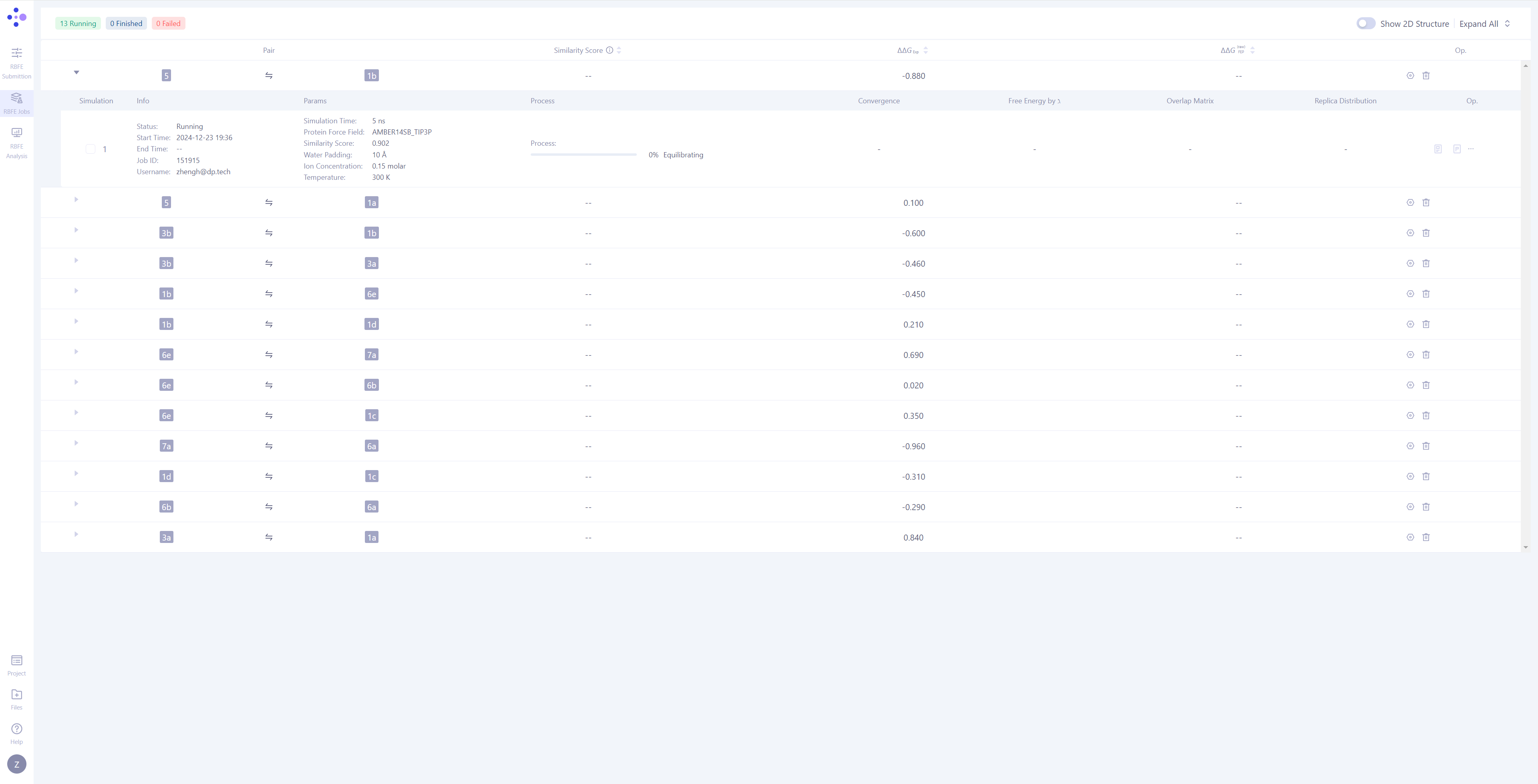
Molecule Pair Grouping in Task Management: In Hermite, FEP tasks are grouped by molecule pairs, with each independent simulation task being the smallest unit of management. Expand Task Details: Click the triangle arrow on the left side of each molecule pair to expand and display the detailed simulation information for that molecule pair. Once expanded, you can view basic information, simulation parameters, task progress, result illustrations, and corresponding operation buttons. Monitor Task Progress: Tasks have three possible statuses: Waiting, Equilibrating, and Production. For tasks in the simulation phase, you can observe their progress and expected completion time.

2.7.2 Analyzing the Calculation Result of a Single Molecular Pair

After the FEP calculation for a single molecule pair is completed, you can use a series of visualization and analysis tools to thoroughly interpret the simulation result and assess the accuracy and reliability of the calculation. This section will guide you on how to interpret and analyze the results of a single molecule pair.

Operation Description	Interface Screenshot
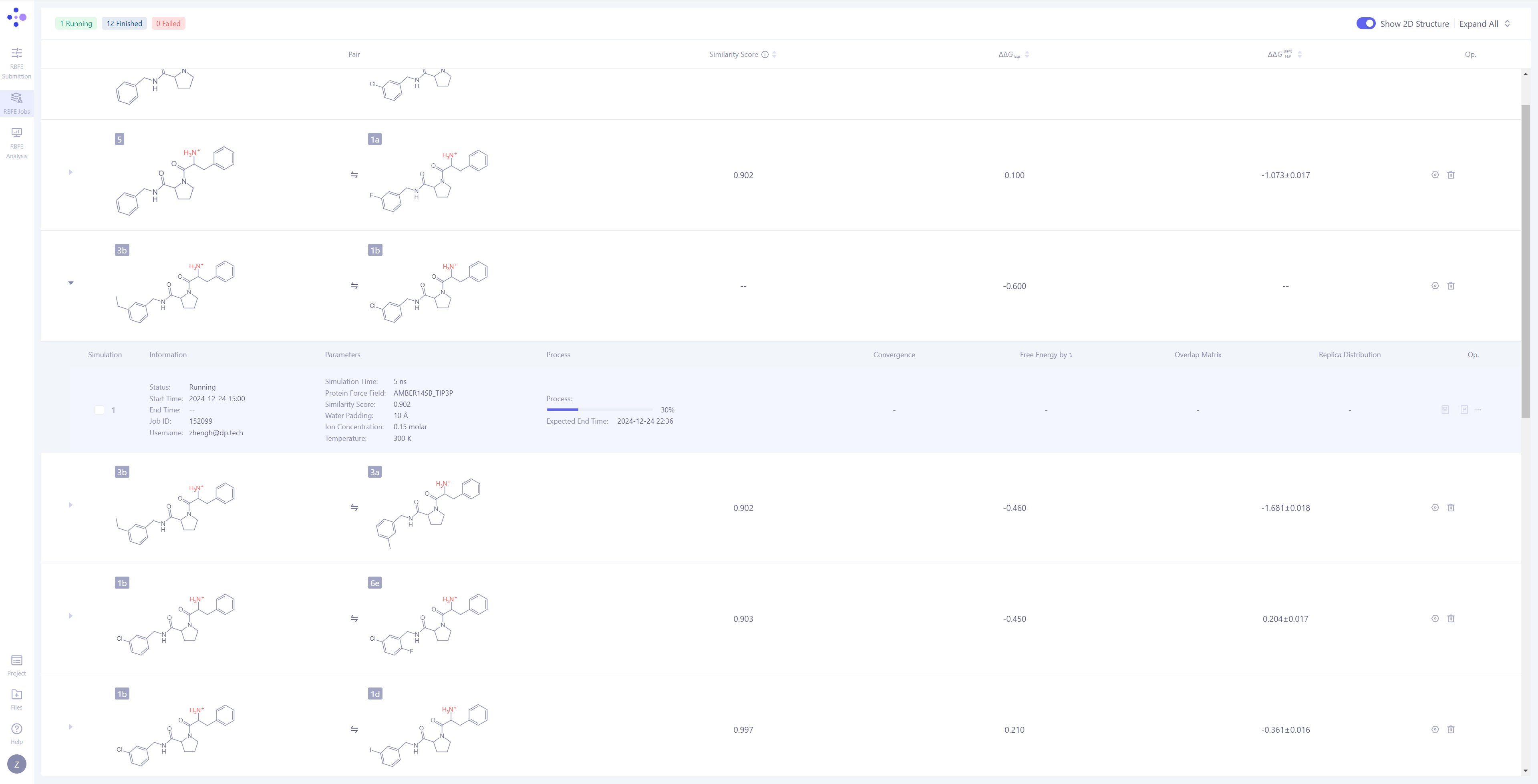
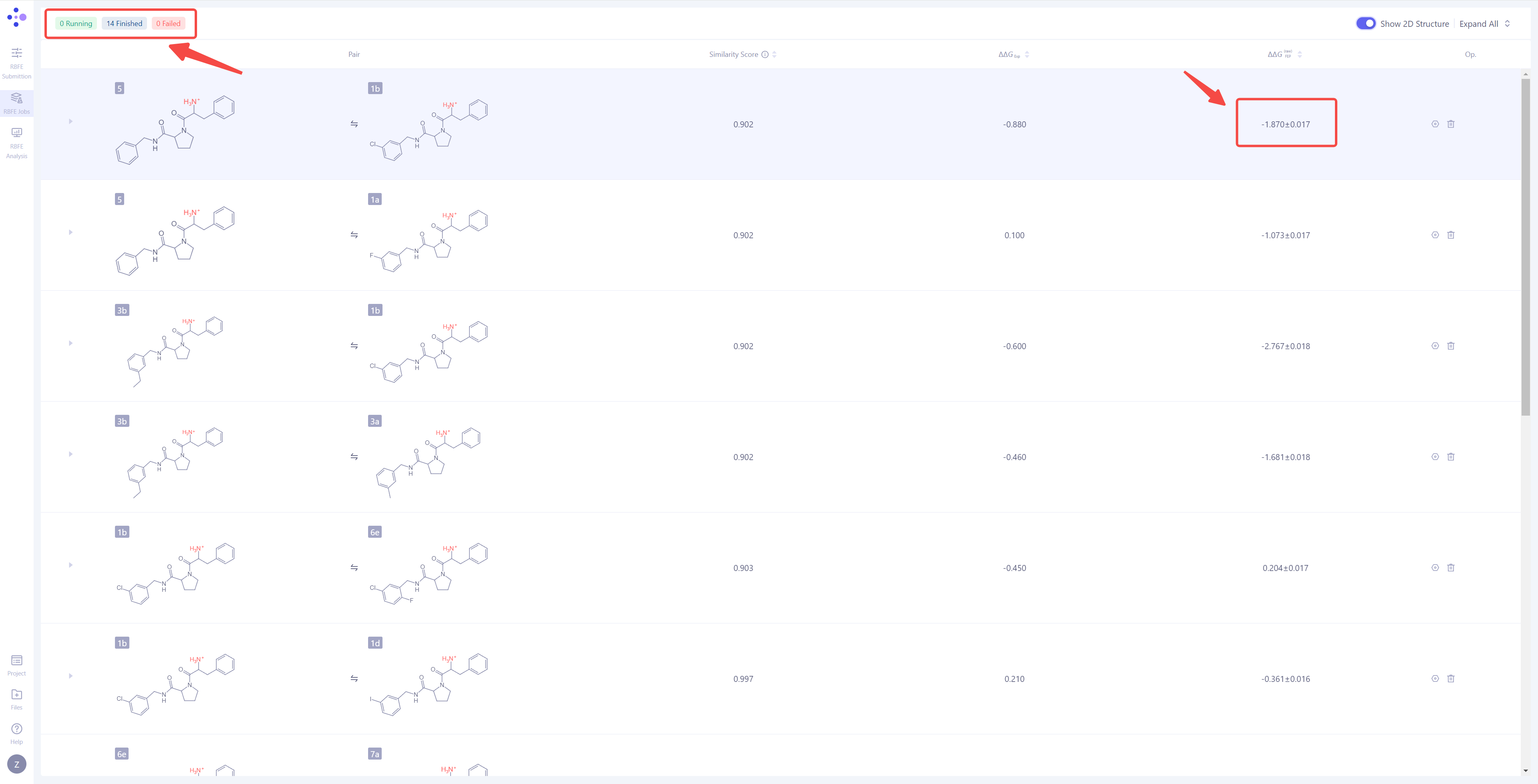
View Calculation Results: When a single simulation task is completed, the status "Task Completed" will be displayed in the upper-left corner. Additionally, the ΔΔG_FEP value for that molecule pair will be automatically calculated and displayed on the interface, representing the predicted binding free energy difference for the molecule pair.
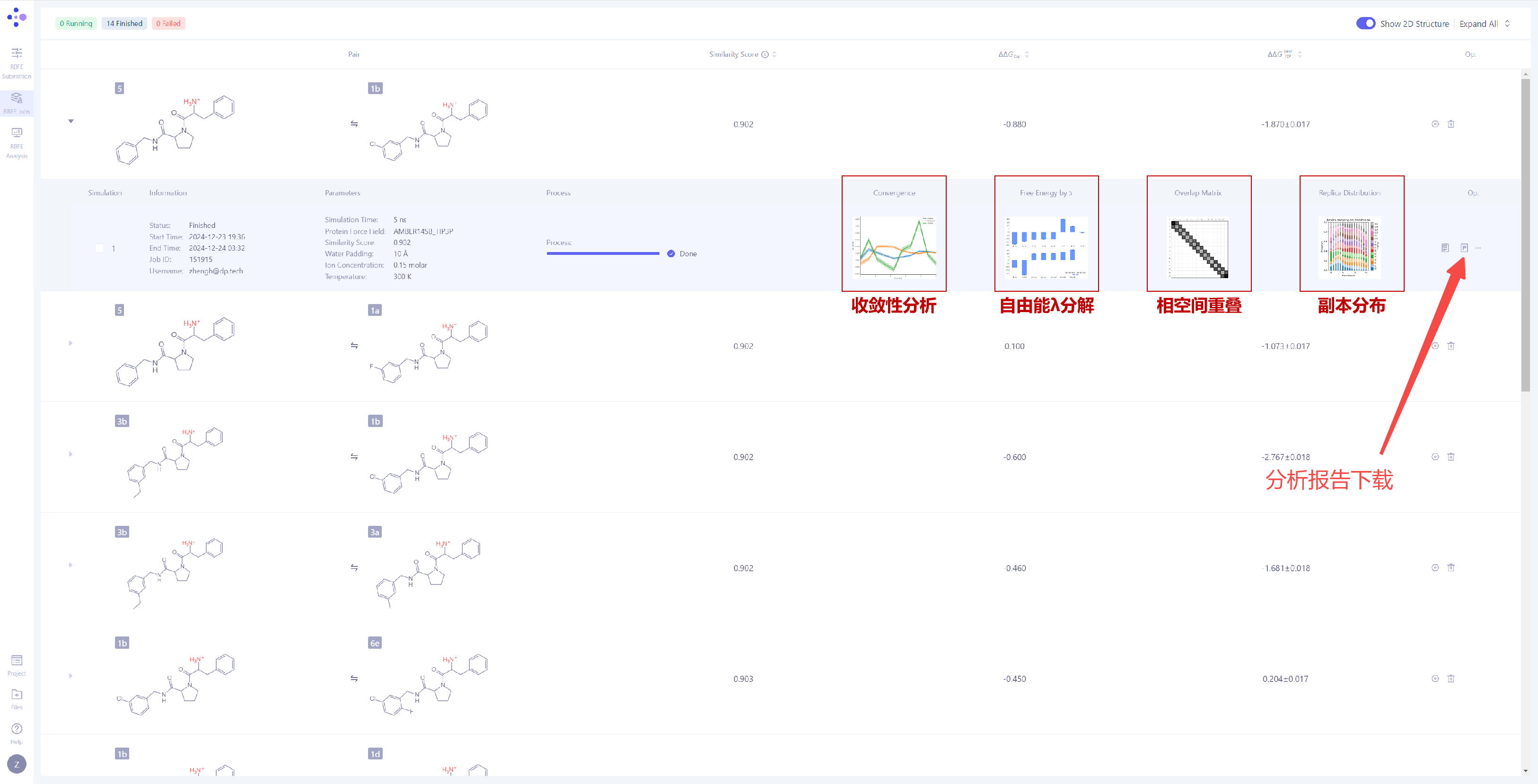
Analyze Simulation Convergence: Expand the task details to observe the simulation convergence for the current FEP calculation. The system provides the following four key analysis charts: Convergence Analysis: This chart shows the difference between the forward and thereverse free energy calculation results, which reflects the extent of hysteresis. Ideally, the difference between forward and reverse results should be small, indicating that the system has fully converged and sampling deviations are negligible. A large difference usually means insufficient state overlap or inadequate sampling. In addition, a smooth and stable moving average suggests that the free energy value has converged, while a continuously changing moving average indicates that the system is not fully converged and still evolving. λ Decomposition of the Free Energy: The λ decomposition of free energy shows the free energy change across different λ states in the system. If ΔΔG values change smoothly across different λ values, it indicates that the system has a stable transition during the alchemical transformation process. Abrupt jumps at certain λ values may indicate critical transition points, insufficient sampling, or system instability. Phase Space Overlap: The phase space overlap matrix displays the conformational sampling overlap between different λ states. The value in each cell represents the overlap of the conformational space between two adjacent λ windows. A higher value (usually recommended to be greater than 0.15) indicates smoother transitions between adjacent states, making the calculation results more reliable. Low overlap in certain regions may suggest significant energy barriers or insufficient sampling between states. Replica Distribution: The replica distribution shows the sampling coverage across different λ states. A uniform distribution indicates that all λ states have been sufficiently sampled, and the sampling is stable and even across all intervals. An uneven distribution may suggest sampling bottlenecks or energy barriers in certain λ intervals, which can affect the accuracy of the final free energy. More detailed analysis results can be obtained by clicking "Report" to download the full report file for in-depth analysis.
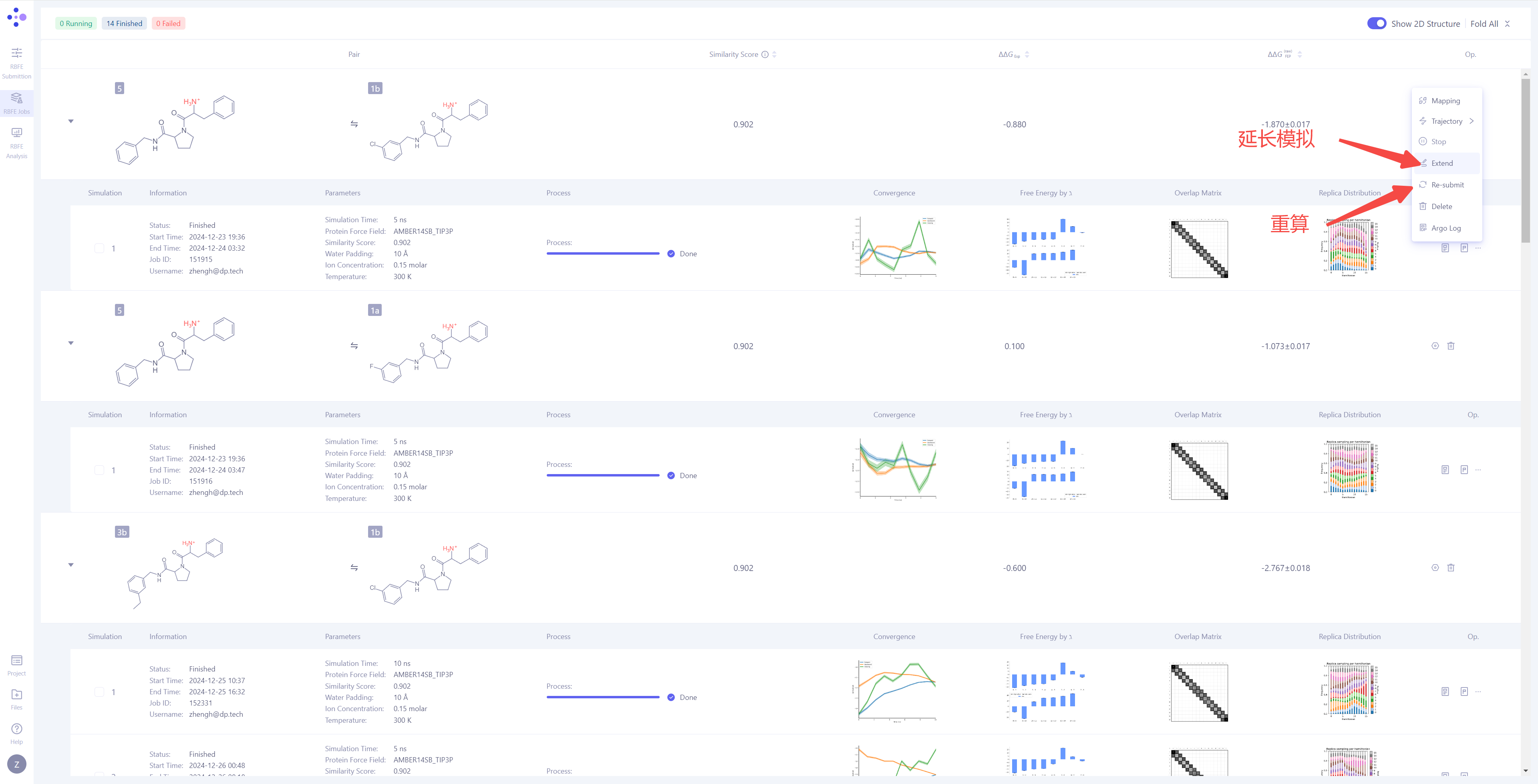
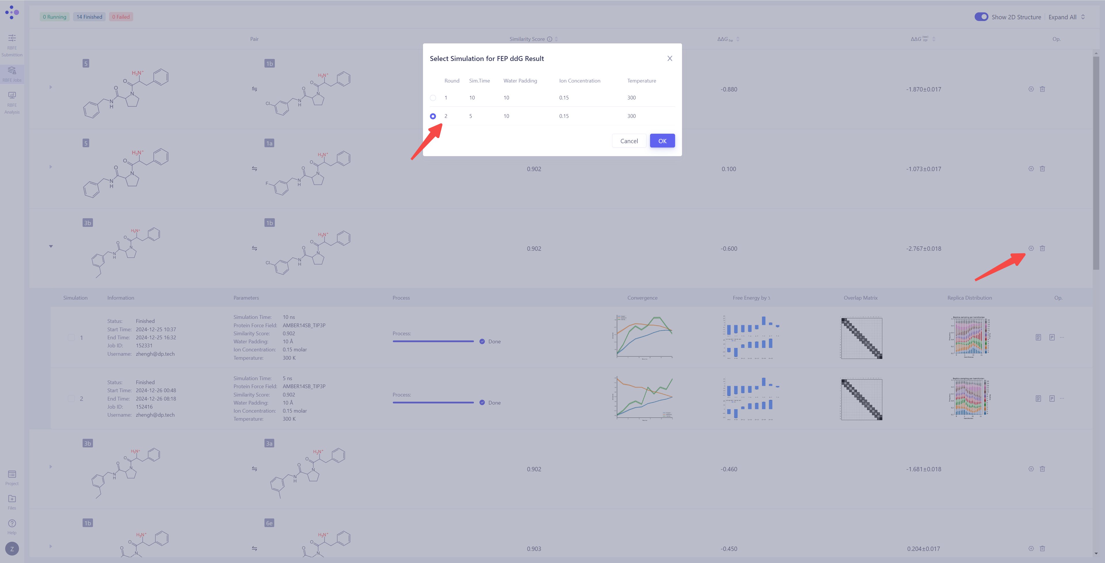
Handling Non-Convergent or Unsatisfactory Results: If you find that the simulation result have not converged or are unsatisfactory, you can click the "Extend" button to extend the simulation time and increase sampling to improve the result stability. If you need to re-run the calculation, you can click the "Re-submit" button to restart the simulation task for that particular molecule pair. When there are multiple simulation results for a molecule pair, you can select a specific simulation as the final source for the ΔΔG_FEP calculation (the system defaults to the most recent simulation result).

2.7.3 Summarizing the Calculation Results for All Molecule Pairs (TBD)

Operation Description	Interface Screenshot
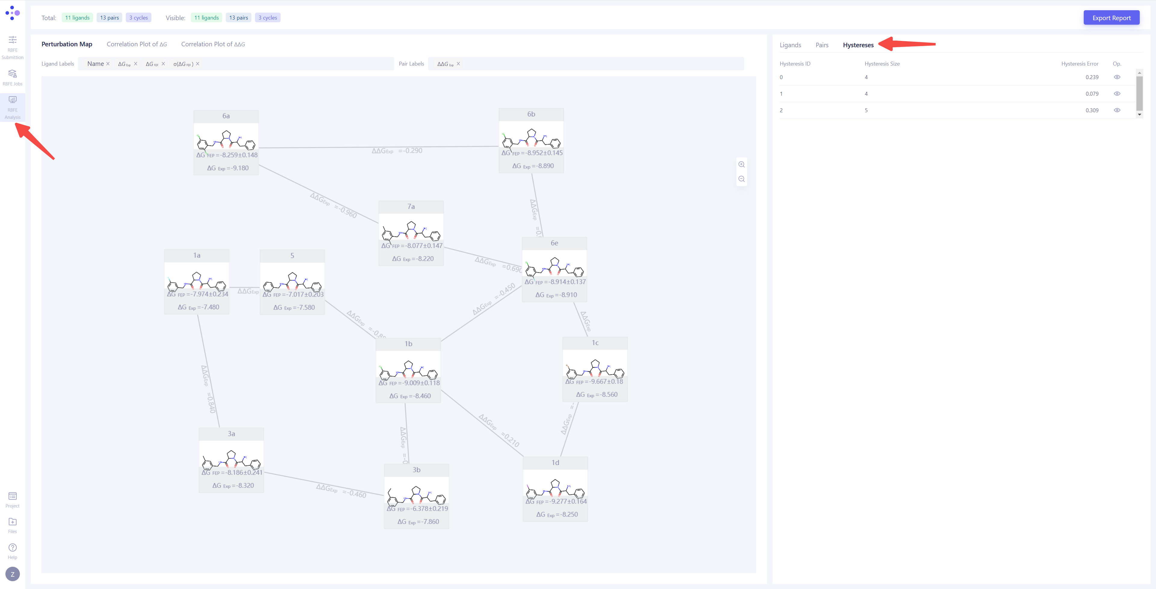
Enter the analysis interface: Once all the molecule pair calculations are completed and the simulation results for each molecule pair have converged, click "RBFE Analysis" in the left sidebar to enter the overall result analysis interface. In this interface, users can conduct systematic analysis based on thermodynamic cycle consistency, ΔΔG correlation, and ΔG correlation.
Thermodynamic Cycle Consistency Analysis: First, select the "Hystereses" view to analyze the thermodynamic cycle consistency of the simulation results. The thermodynamic cycle error (Hystereses Error) reflects the calculation error in the thermodynamic cycle, and ideally, this error should be close to 0. Generally, when the hystereses error is smaller 0.8, the thermodynamic cycle is considered reliable. If the error is large, it is recommended to check the molecule pairs involved in the thermodynamic cycle, extend the simulation time for non-converging molecule pairs, or re-submit the calculations.
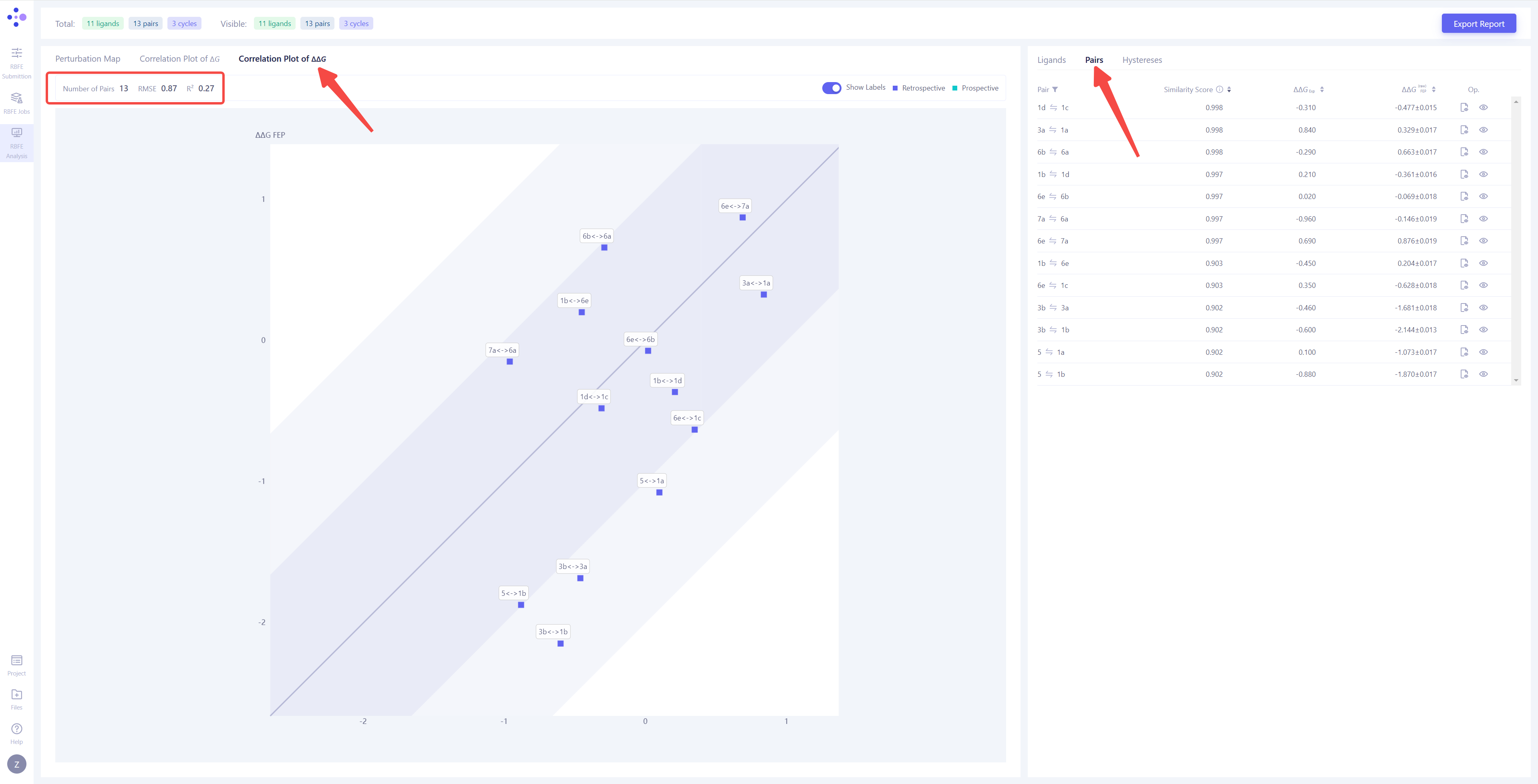
Correlation Analysis of Molecule Pair Calculation Results: Switch the left view to "Correlation Plot of ΔΔG" and the right view to "Pairs" to analyze the FEP calculation results for each molecule pair. In the correlation plot, the x-axis represents the experimental ΔΔG values, while the y-axis represents the ΔΔG values calculated by FEP. The dark-colored area indicates an error range of <1 kcal/mol, and the light-colored area indicates an error range of <2 kcal/mol. The closer the points locate along the diagonal line, the more accurate and reliable the calculation results are. If any molecule pair falls outside the 2 kcal/mol error range, it is recommended to re-run the corresponding FEP calculations to improve the prediction accuracy.
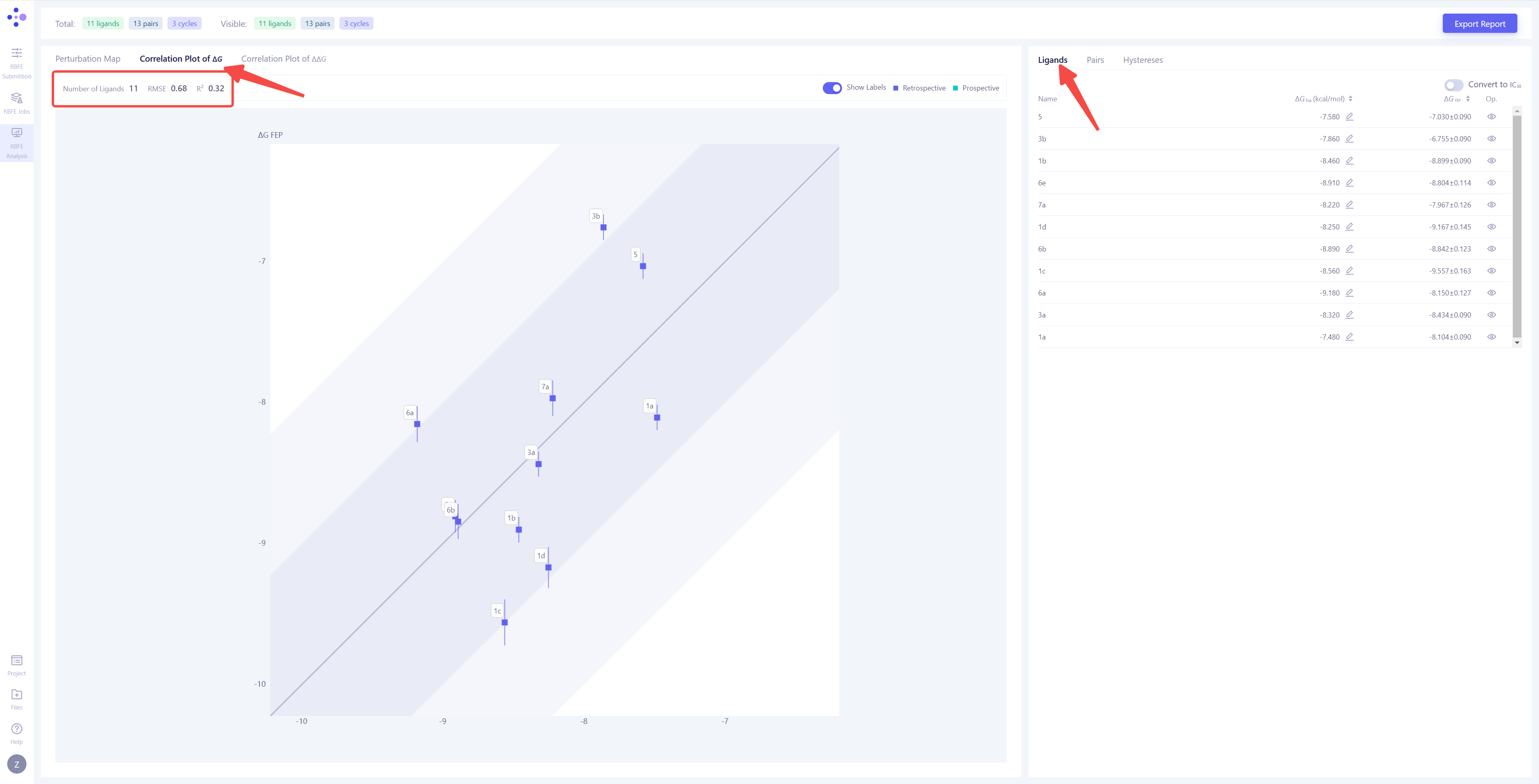
Correlation Analysis of Overall Calculation: Switch the left view to "Correlation Plot of ΔG" and the right view to "Ligands" to conduct a comprehensive analysis of each molecule's FEP calculation result. The overall FEP calculation's correlation coefficient (R²) and root mean square error (RMSE) will be displayed in the upper left corner. When the span of the molecule's experimental activity values is large, it is recommended to refer to the R² value. The closer R² is to 1, the more accurate the calculation results are, with R² > 0.4 being considered 'acceptable'. When the molecule activity values are similar, it is recommended to refer to the RMSE value. The smaller the RMSE, the better the calculation results, with RMSE < 1.4 kcal/mol being an acceptable range.
Confirming the Reliability of the FEP Model: Through the analysis of thermodynamic cycle consistency, ΔΔG correlation, and ΔG correlation, if all the indicators meet expectations, it can be concluded that the FEP calculation result is reliable. The constructed FEP model has reached production level and can be used for predicting the activity of molecules with undetermined activity.

3. Advanced Tricks

1. Why Construct Intermediate Molecules When There Exist Significant Structural Differences Between Two Molecules?
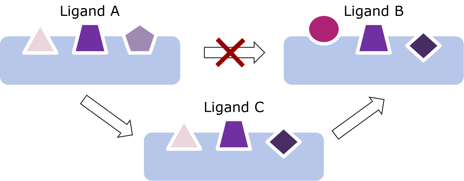
When there are significant structural differences in the scaffold or functional group between two molecules, directly calculating the free energy difference often leads to complex atom mapping relationships and insufficient sampling, which can result in large fluctuations or difficulty in convergence. To allow the system to transit gradually through the alchemical process, it is recommended to manually or automatically generate several intermediate molecules in Uni-FEP, breaking down large structural changes into smaller steps. For example, if molecule A and molecule B differ in two functional groups (referred to as R1 and R2), directly converting A to B could cause a sudden large change to the system, making the atom mapping complex and the sampling insufficient. In this case, one or more intermediate molecules can be constructed: for instance, you can first obtain an intermediate molecule by changing only R1 of A to R1 of B (while keeping R2 unchanged); then, on the basis of C, change R2 to R2 of B. This two-step approach completes the A→B transition, whose calculation is very likely easier to converge than a direct one-step transition. In Uni-FEP, you can create and upload these intermediate molecules, allowing the software to perform the free energy calculation in steps and significantly improving accuracy and reducing computational risks.

2. How to Use Other Similar Molecules as References When the Alignment Between a Candidate Molecule and the Reference Molecule Is not Ideal?
If two molecules cannot achieve a stable and comparable initial conformation through the ligand alignment module, you can select an intermediate molecule that is the most similar to both molecules' scaffold or functional groups as the alignment reference. Then, align the candidate molecule and the reference molecule to this intermediate molecule. For example, if molecule A is monocyclic and molecule B is polycyclic, direct alignment between the two often leads to misalignment or rotational mismatches. If there is an intermediate molecule C in the system (for instance, one whose scaffold is closer to B but with functional groups similar to A), you can first align A with C using Uni-FEP, then align B with C, specifying C as the common reference in the mapping settings. This often provides a more reliable initial conformation, preventing large-scale rearrangements or non-convergence in subsequent FEP calculations.

3. What Atoms or Functional Groups Should Be Focused on When Inpescting the Atom Mapping?
In FEP calculations, mapping incompatible fucntional groups often leads to sharp increases in energy or "atomic crossover." (1) When converting between aromatic rings and aliphatic rings, ensure that a planar benzene ring is not aligned into the non-planar conformation of cyclohexane. If you find that the automated atom mapping causes the rings to interlock, you can manually specify the mapping of carbon atoms on the rings using the software's "Edit Mapping" function. (2) For linear cyano groups (-CN), if the target molecule contains functional groups like -NO₂ or -NH₂, which have vastly different physicochemical properties, it is best to construct one or more transition molecules before proceeding with the main calculation to avoid significant electronic structure changes in a single step. Additionally, for molecules with chiral centers, ensure that the R/S configuration is not flipped by the automatic atom mapping. If you observe stereochemical inversion, manually modify the atom mapping and verify it through the visualization interface.

4. How to Determine the Protonation State of Key Residues Based on the Protein-Ligand Binding Pose?
Protonatable amino acids in proteins (such as histidine, lysine, glutamic acid, etc.) often alter their protonation state under physiological conditions due to the local environment created by the ligand. (1) If the ligand has a positively charged group that is spatially adjacent to the histidine side chain but lacks a clear hydrogen bond, consider whether the histidine still tends to be protonated to form an electrostatic attraction with the ligand. Conversely, if a carboxyl group of the ligand is within 3 Å of the glutamic acid side chain and forms a stable hydrogen bond or salt bridge, glutamic acid is more likely to be in its deprotonated state. (2) In practice, you can combine the software's pKa predictions, distance analysis, and crystal structure information. If the automatically assigned protonation state does not match the known binding mode, manually correct the protonation state of the residue and maintain consistent across all subsequent calculations for the protein.

5. Why Removing Unnecessary Perturbation Edges Based on Thermodynamic Cycles?
When comparing relative free energy differences between multiple molecules, a network of nodes (A, B, C, D, for instance.) connected by edges is often formed. If an edge (such as A→D) involves changing multiple functional groups simultaneously or has poor atom mapping, it may introduce convergence difficulty or large fluctuation. (1) In such cases, you can first proceed with smoother transitions like A→B, B→C, C→D, where each step involves a reasonable and easily-converging transition, and then use thermodynamic cycles to derive the result for A→D. (2) If, after evaluation, certain edges consistently introduce errors, it may be better to simply remove them from the calculation network and retain edges with better cycle closure. This can reduce computational load and improve the overall prediction accuracy.

4. Common Issues

Tip: If you have any questions that are not covered here, feel free to contact us! You can directly reach out to your assigned sales representative or send your inquiry to help@dp.tech.

1. What is the Difference Between FEP and MM-GB/PBSA in Principle?
FEP directly calculates the free energy difference (ΔΔG) between two states using molecular dynamics simulations and free energy perturbation methods, eliminating biases during energy minimization via thermodynamic paths. MM-GBSA and MM-PBSA, on the other hand, are based on single-point energy calculations, estimating the free energy by placing molecules in generalized Born or Poisson-Boltzmann solvent models. FEP is more accurate but computationally expensive, while MM-GB/PBSA is better suited for rapid screening.

2. When There Exist Multiple Amino Acid Chains in a Protein, Which Chains Shoule be Kept?
Typically, only the amino acid chains that interact with the ligand need to be retained, while chains could be removed to improve computational efficiency. However, it is important to note that changes in the ligand structure might cause previously non-interacting amino acid chains to form interactions. Therefore, it is recommended to thoroughly check all potential interactions between the ligand and amino acids before the calculation to ensure the selected chains accurately reflect the key interactions in the system.

3. Should Water Molecules in the Protein Crystal Structure be Retained During Protein Preparation?
It is generally recommended to retain the following types of water molecules in the crystal structure:(1) Water molecules that form key interactions with the protein-ligand complex, such as those involved in hydrogen bonding or other non-covalent interactions. (2) Water molecules that significantly contribute to the stability of local protein regions, such as those maintaining the active site structure or critical secondary structures.
Other less important water molecules can be removed to simplify the system and improve computational efficiency. It is recommended to assess the necessity of retaining water molecules based on the crystal structure and simulation requirements.

4. What Should be Considered When Performing FEP Calculations on Membrane Protein Systems?
To preserve the biological environment as much as possible, it is essential to carry out the calculation in a membrane environment constructed by POPC when performing FEP calculations on membrane protein systems. Therefore, the protein should be embedded in the membrane; otherwise, the accuracy of the results may be affected, or the task may even fail. Additionally, due to the higher number of atoms in membrane-bound systems and the need for equilibration in large-scale MD simulations, the computational load of FEP on membrane systems is typically 2 to 3 times greater than proteins in the apo environment. Consequently, task runtime will be longer, and computational resources should be planned accordingly.

5. Any Special Treatments for Charged Small Molecules during FEP Calculations?
If ligands involved in the FEP calculation have the same net charge (e.g., both are neutral), no extra actions is needed other than ensuring that the chemical structure and charge of each ligand are accurate. However, if the net charge of the ligand changes (e.g., a change of +1 in the net charge) in a molecule pair, Uni-FEP employs special algorithms to maintain charge balance in the system during MD simulations. This is typically achieved by gradually converting water molecules into positive and negative ions. Additionally, adding appropriate amounts of cations and anions can further stabilize the calculation.

6. What is the Relationship Between Molecular Affinity Values and Binding Free Energy?
The relationship between the molecular affinity (e.g., IC₅₀, Kᵢ, or Kd values) and the binding free energy (ΔG) can be approximately calculated using the following formula (1), where R is the idea gas constant, T is the temperature (typically 298K). Using this formula, the mmolecular affinity value can be converted to the corresponding ΔG value. Notably, every 1kcal/mol change in ΔG conrresponds to a change of 6 times difference in the molecualr affinity. Therefore, minor differences in the binding free energy can reflect significant differences to teh binding affinity. When applying this formula, make sure that the molecular affinity measurement is acquired under similar experimental conditions and is measured on a cell level; otherwise, the above conversion can be mistaken. Through this conversion, the ΔG value computed by FEP can be compared directly to the experimental result, hence better assessing the prediction accuracy of the FEP computational mocel.

$$\Delta G=RT\ln K_{d}=-RT\cdot pIC_{50} \tag{1}$$

7. Generally, What Range of RMSE and R² Values Indicates Good FEP Calculation Results?
When there is a large span in experimental affinity values of the molecules, it is recommended to refer to the R² value. The closer R² is to 1, the more accurate the calculation results, and typically, results with R² greater than 0.4 are considered acceptable. When the affinity values of the molecules are similar, it is better to refer to the RMSE value. The smaller the RMSE, the better the calculation results. Generally, an RMSE value under 1.4 kcal/mol is considered acceptable for FEP.

8. How to Interpret the Thermodynamic Cycle in the Results?
A thermodynamic cycle is formed through the calculation of ΔΔG. For example, if three molecules are included in a task, forming a cycle of A→B, B→C, C→A, the thermodynamic principle suggests that the thermodynamic cycle error should theoretically be 0. Therefore, the smaller the absolute value of the thermodynamic cycle error, the more reliable the pairwise calculation results involved in the cycle. Larger thermodynamic cycle errors may indicate calculation biases or imbalances in the system, and further examination of the system setup or simulation parameters may be necessary.

9. Can FEP be Used to Predict Agonist Activity?
Binding free energy is a necessary but insufficient condition for agonist activity. An agonist must first stably bind to the target protein (indicated by a low binding free energy, ΔG), and upon binding, it induces specific conformational changes that trigger signal transduction. In conclusion, binding is a prerequisite for agonist activity. Therefore, highly active molecules should at least demonstrate good binding affinity.

5. Benchmark Tests

The benchmark test aims to systematically evaluate the performance of the Free Energy Perturbation (FEP) method in drug discovery, verifying its accuracy, stability, and applicability in predicting binding free energies across various scenarios. Similar to the validation phase in actual drug discovery projects, benchmark tests is performed on widely validated and publicly reported standard datasets. Through a unified testing process and evaluation metrics, benchmark tests demonstrate the method’s overall performance across different targets and chemical transformation scenarios.

In terms of result interpretation, as discussed earlier, when the experimental values for molecular affinity span a wide range, R² (correlation coefficient) is more suitable as an evaluation metric. The closer R² is to 1, the stronger the correlation between the predicted results and experimental data, with R² > 0.4 generally considered acceptable. When the molecular affinity values are relatively close, RMSE (root mean square error) becomes more valuable as a reference. A lower RMSE indicates smaller prediction errors, with RMSE < 1.4 kcal/mol considered good predictive performance.

In the below section, we showcase Uni-FEP's performance on three publicly availiable benchmarks and compare them with the reported values in the literatures. Through these benchmark tests, we demonstrate Uni-FEP's state-of-the-art performance across different systems and scenarios as well as identify potential limitations on certain systems, and ultimately provide a scientific basis for subsequent algorithm optimization and drug discovery efforts.

5.1 The S Benchmark

The S Benchmark Test is a highly precise and systematic dataset specifically designed to assess the broad applicability of the Free Energy Perturbation (FEP) method in drug discovery. This benchmark covers eight classic drug development targets, including protein kinases, enzymes, and receptors. It also includes eight types of chemical transformation scenarios, such as charge changes, scaffold hopping, and ring structure conversions, addressing typical and challenging issues encountered in drug design. The testing process provides detailed protein-ligand preparation guidelines, ligand modeling methods, and standardized computational settings, offering comprehensive support for researchers to evaluate and optimize the FEP method in real-world scenarios.

Series	Num. Compounds	Num. Perturbations	Hermite®️ Uni-FEP (5ns)		Reference[1] (5ns)
			R²	RMSE kcal/mol	R²	RMSE kcal/mol
BACE	36	58	0.47	0.80	0.39	1.08
CDK2	16	25	0.54	0.81	0.42	1.31
JNK1	21	31	0.59	0.65	0.71	0.83
MCL1	42	71	0.57	1.19	0.49	1.24
P38	34	56	0.42	0.92	0.49	1.16
PTP1B	23	49	0.57	0.91	0.85	0.74
Thrombin	11	16	0.86	0.60	0.68	0.79
Tyk2	16	24	0.63	0.81	0.86	0.69
Average	-	-	0.58	0.84	0.61	0.98

5.2 The M Benchmark

The M Benchmark Test is a well-designed and comprehensive dataset focused on evaluating the performance of the Free Energy Perturbation (FEP) method in complex drug design scenarios. This benchmark selects eight representative drug targets and includes 264 ligands, covering chemical transformation scenarios such as charge changes, ring structure conversions, and scaffold hopping to simulate the diverse needs of drug discovery. The test provides detailed protein structure preparation and ligand modeling processes, aiming to promote the practical application of the FEP method in drug development through systematic validation.

Series	Num. Compounds	Num. Perturbations	Hermite®️ Uni-FEP (5ns)		Reference[1] (5ns)
			R²	RMSE kcal/mol	R²	RMSE kcal/mol
CDK8	32	54	0.65	1.02	0.56	1.63
c-Met	24	40	0.69	1.12	0.82	1.07
Eg5	28	51	0.22	1.30	0.35	1.25
HIF-2α	41	103	0.32	1.36	0.61	1.10
PFKFB3	40	136	0.16	1.46	0.58	1.42
SHP-2	26	39	0.02	1.82	0.50	1.60
SYK	46	101	0.59	1.18	0.51	1.05
TNKS2	27	52	0.30	1.01	0.29	1.61
Average	-	-	0.37	1.28	0.53	1.34

5.3 The GPCR-FEP Benchmark

The GPCR-FEP Benchmark Test is one of the most comprehensive datasets currently available for G Protein-Coupled Receptors (GPCRs), specifically designed to assess the performance of the Free Energy Perturbation (FEP) method on membrane protein targets. This benchmark covers eight GPCR targets, twelve protein systems and a total of 139 ligands, and provides detailed guidance on protein-ligand structure preparation, water distribution schemes, and membrane environment construction methods. By accurately reproducing the complexity of membrane protein systems, this benchmark provides researchers with high-quality data and a standardized computational framework on GPCR systems, advancing the application of FEP technology in GPCR-targeted drug discovery.

Series	Num. Compounds	Num. Perturbations	Hermite®️ Uni-FEP (5ns)		Reference[2] (5ns)
			R²	RMSE kcal/mol	R²	RMSE kcal/mol
A2A-D	10	14	0.83	0.76	0.9	1.00
A2A-L	7	10	0.84	0.54	0.58	0.97
A2A-M	9	17	0.50	0.91	0.61	0.66
A2A-P	7	10	0.33	0.38	0.3	0.35
OX2-set1	27	40	0.57	0.88	0.65	1.05
OX2-set2	24	39	0.25	1.07	0.62	0.84
CXCR4	9	16	0.44	1.10	0.2	1.21
β1	9	16	0.14	0.91	0.15	0.75
δ	11	19	0.59	0.83	0.71	0.54
Average	-	-	0.50	0.82	0.51	0.82

Series	Num. Compounds	Num. Perturbations	Hermite®️ Uni-FEP (5ns)
			R²	RMSE kcal/mol
mGlu5	12	20	0.74	1.14
D3	6	10	0.67	1.09
TA1	8	15	0.58	1.07
Average	-	-	0.66	1.10

Reference: [1] Ross GA, Lu C, Scarabelli G, Albanese SK, Houang E, Abel R, Harder ED, Wang L. The maximal and current accuracy of rigorous protein-ligand binding free energy calculations. Communications Chemistry. 2023 Oct 14;6(1):222. [2] Guo Y, Zhou Y, Bai Q, Bo Z, Song K, Chang J, Zhang Y, Yang M, Deng Y, Wang D. A Benchmark for Accurate GPCR Ligand Binding Affinity Prediction with Free Energy Perturbation. ChemRxiv, 2023.